Summary
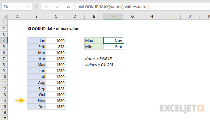
To use XLOOKUP to find the date of the max value, you can use the MAX function with the XLOOKUP function. In the example shown, the formula in F4 is:
=XLOOKUP(MAX(values),values,dates)
where values (C4:C15) and dates (B4:B15) are named ranges.
Generic formula
=XLOOKUP(MAX(values),values,dates)
Explanation
This formula is based on the XLOOKUP function. Working from the inside out, we use the MAX function to calculate a lookup value:
MAX(values)
MAX is nested inside XLOOKUP, and returns a value directly as the first argument:
=XLOOKUP(MAX(values),values,dates)
- The lookup_value is delivered by MAX
- The lookup_array is the named range values (C4:C15)
- The return_array is the named range dates (B4:B15)
- The match_mode is not provided and defaults to 0 (exact match)
- The search_mode is not provided and defaults to 1 (first to last)
Without named ranges
The example uses named ranges for convenience and readability. Without named ranges, the same formula is:
=XLOOKUP(MAX(C4:C15),C4:C15,B4:B15)
Min value
To return the date of the minimum value, the formula in F5 just substitutes the MIN function for the MAX function:
=XLOOKUP(MIN(values),values,dates)
With INDEX and MATCH
The equivalent INDEX and MATCH formula to return the date of max value is:
=INDEX(dates,MATCH(MAX(values),values,0))
Note: although the example uses a vertical range of data, both formulas above will work just as well with a horizontal range.