XLOOKUP horizontal lookup

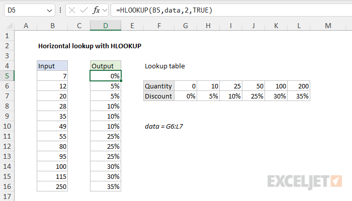
In this example, the goal is to perform a horizontal lookup to determine the correct quantity-based discount. The range G6:L7 contains quantity-based discounts. Column B contains random quantities used when testing the formula. This problem can be easily solved with the XLOOKUP function or the HLOOKUP function. Both methods are explained below.

XLOOKUP formula

One of XLOOKUP's nice benefits is its ability to work with vertical or horizontal data. The syntax used for horizontal lookups is the same as for vertical lookups. In the worksheet shown, the formula in cell D5, copied down, is:

=XLOOKUP(B5,quantity,discount,,-1)

Where quantity (G6:L6) and discount (G7:L7) are named ranges used for convenience and readability only. The same formula without named ranges looks like this:

=XLOOKUP(B5,$G$6:$L$6,$G$7:$L$7,,-1)

Note that the lookup_array and return_array are both provided as absolute references to lock these ranges as these formulas are copied down. This is not required with named ranges because they automatically behave as absolute references.

XLOOKUP's arguments are configured as follows:

• The lookup_value comes from cell B5
• The lookup_array is the named range quantity (G6:L6)
• The return_array is the named range discount (G7:L7)
• The not_found argument is omitted
• The match_mode is set to -1 (exact match or next smaller)
• The search_mode is omitted and defaults to 1 (first to last)

At each row, XLOOKUP looks up the quantity in column B. If an exact match is found, the corresponding discount in row 7 is returned. When an exact match is not found, the discount associated with the next smallest quantity is returned. 

HLOOKUP formula

Working with HLOOKUP is similar to working with the VLOOKUP function. Both functions require the entire lookup table as the table_array argument and use an index number to specify return values. However, for VLOOKUP, the index number represents a column number, while for HLOOKUP, the index represents a row number. This problem can also be solved with the HLOOKUP function like this:

=HLOOKUP(B5,data,2,TRUE)

Where data is the named range G6:L7.

In the formula above, the arguments are configured like this:

• The lookup_value comes from cell B5
• The table_array is provided as data (G6:L7)
• The row_index_num is provided as 2 since discounts are in the second row.
• The range_lookup argument is provided as TRUE to explicitly enable an approximate match.

Named ranges automatically behave like locked references when copied. Without named ranges, the same formula would need an absolute reference for the lookup table like this:

=HLOOKUP(B5,$G$6:$L$7,2,TRUE)

The absolute reference prevents table_array from changing as the formula is copied down the table. 

XLOOKUP vs HLOOKUP

When we compare the XLOOKUP formula to the HLOOKUP formula, there are several differences worth noting:

• HLOOKUP requires the full table array. XLOOKUP requires only the range that contains lookup values.
• HLOOKUP requires a row index to specify a result column. XLOOKUP requires a range that contains result values.
• HLOOKUP performs an approximate match by default. XLOOKUP performs an exact match by default, so we must set match_mode to -1 (exact match or next smaller).
• HLOOKUP requires lookup data to be sorted by lookup value. XLOOKUP works with unsorted data.
• HLOOKUP performs horizontal lookups only. XLOOKUP can perform both horizontal and vertical lookups.

INDEX and MATCH

Naturally, you can also solve this problem with INDEX and MATCH, the Swiss Army Knife of lookup formulas :) With named ranges, the formula will look like this:

=INDEX(discount,1,MATCH(B5,quantity,1))

I've included all three options on different sheets. Download the workbook and try it out yourself.