=HLOOKUP(lookup_value, table_array, row_index, [range_lookup])- lookup_value - The value to look up.
- table_array - The table from which to retrieve data.
- row_index - The row number from which to retrieve data.
- range_lookup - [optional] A Boolean to indicate exact match or approximate match. Default = TRUE = approximate match.
Using the HLOOKUP function
The HLOOKUP function can locate and retrieve a value from data in a horizontal table. Like the "V" in VLOOKUP which stands for "vertical", the "H" in HLOOKUP stands for "horizontal". The lookup values must appear in the first row of the table, moving horizontally to the right. HLOOKUP supports approximate and exact matching, and wildcards (* ?) for finding partial matches.
HLOOKUP searches for a value in the first row of a table. When it finds a match, it retrieves a value at that column from the row given. Use HLOOKUP when lookup values are located in the first row of a table. Use VLOOKUP when lookup values are located in the first column of a table.
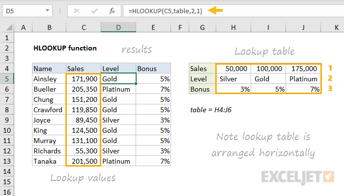
HLOOKUP takes four arguments. The first argument, called lookup_value, is the value to look up. The second argument, table_array, is a range that contains the lookup table. The third argument, row_index_num is the row number in the table from which to retrieve a value. In the example shown, HLOOKUP is used to look up values from row 2 (Level) and row 3 (Bonus) in the table. The fourth and final argument, range_lookup, controls matching. Use TRUE or 1 for an approximate match and FALSE or 0 for an exact match.
Example #1 - approximate match
In the example shown, the goal is to look up the correct Level and Bonus for the sales amounts in C5:C13. The lookup table is in H4:J6, which is the named range "table". Note this is an approximate match scenario. For each amount in C5:C13, the goal is to find the best match, not an exact match. To lookup Level, the formula in cell D5, copied down, is:
=HLOOKUP(C5,table,2,1) // get level
To get Bonus, the formula in E5, copied down, is:
=HLOOKUP(C5,table,3,1) // get bonus
Notice the only difference between the two formulas is the row index number: Level comes from row 2 in the lookup table, while Bonus comes from row 3. The match mode has been set explicitly to approximate match by providing the last argument, range_lookup, as 1.
Example #2 - exact match
In the screen below, the goal is to look up the correct level for a numeric rating 1-4. In cell D5, the HLOOKUP formula, copied down, is:
=HLOOKUP(C5,table,2,FALSE) // exact match
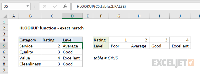
where table is the named range G4:J5. Notice the last argument, range_lookup is set to FALSE to require an exact match.
Notes
- Range_lookup controls whether the lookup value needs to match exactly or not. The default is TRUE = allow non-exact match.
- Set range_lookup to FALSE to require an exact match.
- If range_lookup is omitted or TRUE, and no exact match is found, HLOOKUP will match the nearest value in the table that is still less than the lookup value. However, HLOOKUP will still match an exact value if one exists.
- If range_lookup is TRUE , lookup values in the first row of the table must be sorted in ascending order. Otherwise, HLOOKUP may return an incorrect or unexpected value.
- If range_lookup is FALSE (exact match), values in the first row of the lookup table do not need to be sorted.