Excel GETPIVOTDATA function

Purpose

Retrieve data from a pivot table in a formula

Return value

The data requested

Syntax

=GETPIVOTDATA(data_field,pivot_table,[field1, item1],...)

data_field - The name of the value field to query.
pivot_table - A reference to any cell in the pivot table to query.
field1, item1 - [optional] A field/item pair.

How to use

Use the GETPIVOTDATA function to query an existing Pivot Table and retrieve specific data based on the pivot table structure. The advantage of GETPIVOTDATA over a simple cell reference is that it collects data based on structure, not cell location. GETPIVOTDATA will continue to work correctly even when a pivot table changes, as long as the field(s) being referenced is still present.

The first argument, data_field, names a value field to query. The second argument, pivot_table, is a reference to any cell in an existing pivot table. Additional arguments are supplied in field/item pairs that act like filters to limit the data retrieved based on the structure of the pivot table. For example, you might supply the field "Region" with the item "East" to limit sales data to Sales in the East Region.

The GETPIVOTDATA function is generated automatically when you reference a value cell in a pivot table by pointing and clicking. To avoid this, you can simply type the address of the cell you want (instead of clicking). If you want to disable this feature entirely, disable "Generate GETPIVOTDATA" in the menu at Pivot TableTools > Options > Options (far left, below the pivot table name).

Examples

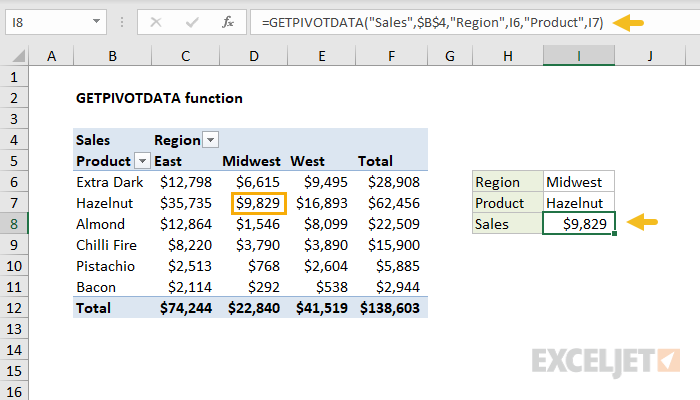
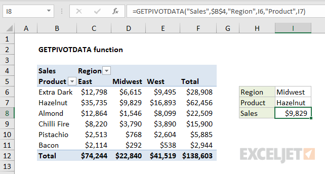
The examples below are based on the following pivot table:

Example of GETPIVOTDATA function with a pivot table

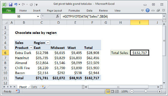
The first argument in the GETPIVOTDATA function names the field from which to retrieve data. The second argument is a reference to a cell that is part of the pivot table. To get total Sales from the pivot table shown:

=GETPIVOTDATA("Sales",$B$4) // returns 138602

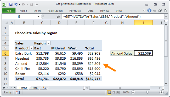
Fields and item pairs are supplied in pairs entered as text values. To get total sales for the Product Hazelnut:

=GETPIVOTDATA("Sales",$B$4,"Product","Hazelnut") // returns 62456

To get total Sales for the West region:

=GETPIVOTDATA("Sales",$B$4,"Region","West") // returns 41518

To get total sales for Almond in the East region, you can use either of the formulas below:

=GETPIVOTDATA("Sales",$B$4,"Region","East","Product","Almond")
=GETPIVOTDATA("Sales",$B$4,"Product","Almond","Region","East")

You can also use cell references to provide field and item names. In the example shown above, the formula in I8 is:

=GETPIVOTDATA("Sales",$B$4,"Region",I6,"Product",I7)

The values for Region and Product come from cells I5 and I6. The data is collected based on the region "Midwest" in cell I6 for the product "Hazelnut" in cell I7.

Dates and times

When using GETPIVOTDATA to fetch information from a pivot table based on a date or time date or time, use Excel's native format, or a function like the DATE function. For example, to get total Sales on April 1, 2021 when individual dates are displayed:

=GETPIVOTDATA("Sales",A1,"Date",DATE(2021,4,1))

When dates are grouped, refer to the group names as text. For example, if the Date field is grouped by year:

=GETPIVOTDATA("Sales",A1,"Year","2021")

Notes

The name of the data_field, and field/item values must be enclosed in double quotes (")
GETPIVOTDATA will return a #REF error if any fields are spelled incorrectly.
GETPIVOTDATA will return a #REF error if the reference to pivot_table is not valid.