Summary
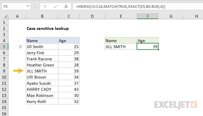
To perform a case-sensitive lookup, you can use the EXACT function with INDEX and MATCH. In the example shown, the formula in F5 is:
=INDEX(C5:C14,MATCH(TRUE,EXACT(E5,B5:B14),0))
This formula returns 39, the age of "JILL SMITH" in uppercase. Notice that the first "Jill Smith" in the list has a different case and is ignored.
Note: this is an array formula and must be entered with Control + Shift + Enter in older versions of Excel.
Generic formula
=INDEX(range1,MATCH(TRUE,EXACT(A1,range2),0))
Explanation
In this example, the goal is to perform a case-sensitive lookup on the name in column B, based on a lookup value entered in cell E5. By default, Excel is not case-sensitive. This means that standard lookup functions like VLOOKUP, XLOOKUP, and INDEX and MATCH are also not case-sensitive. These formulas will simply return the first match, ignoring upper and lower case. The classic way to work around this limitation is to build a lookup formula that incorporates the EXACT function, which performs a case-sensitive comparison. In a nutshell, we use the EXACT function to generate an array of TRUE and FALSE values, then alter the lookup formula to look for the first TRUE value. The article below explains how to use this approach with INDEX and MATCH, and XLOOKUP.
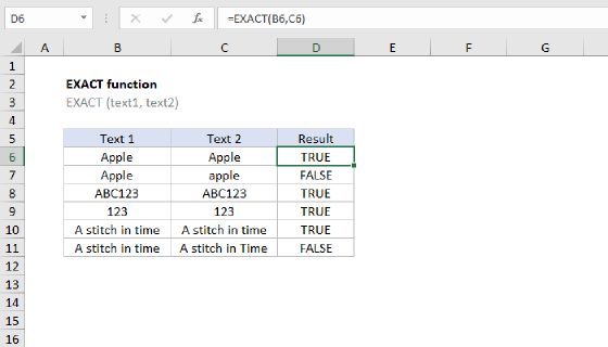
EXACT function
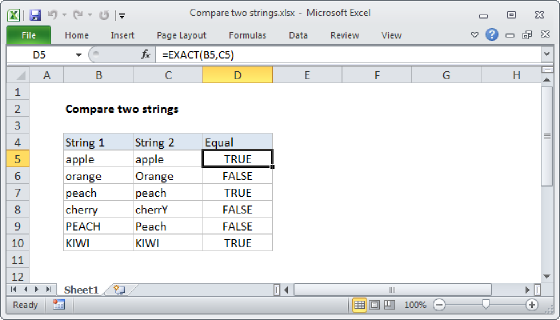
The EXACT function compares two text strings in a case-sensitive fashion. If the two strings are exactly the same, taking into account upper and lower case characters, EXACT returns TRUE. Otherwise, EXACT returns FALSE. For example:
=EXACT("apple","apple") // returns TRUE
=EXACT("Apple","apple") // returns FALSE
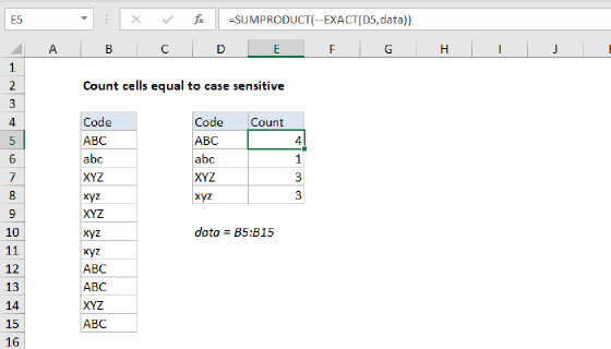
If we use the EXACT function on a range of values, we will get back multiple results. For example, if we use EXACT to compare the value in cell E5 with the range B5:B14:
EXACT(E5,B5:B14)
We get back an array that contains 10 TRUE and FALSE values like this:
{FALSE;FALSE;FALSE;FALSE;TRUE;FALSE;FALSE;FALSE;FALSE;FALSE}
This is because we are checking the name in E5 ("JILL SMITH") against all 10 names in the range B5:B14. Notice the only TRUE value is in the 5th position. This corresponds to cell B9, which contains "JILL SMITH".
INDEX and MATCH solution
In the worksheet shown, the formula in cell F5 is:
=INDEX(C5:C14,MATCH(TRUE,EXACT(E5,B5:B14),0))
Working from the inside-out, EXACT is configured to compare the value in E5 against all names in the range B5:B14:
EXACT(E5,B5:B14) // returns 10 results
The EXACT function performs a case-sensitive comparison and returns TRUE or FALSE as a result. Because we are checking the name in E5 ("JILL SMITH") against all 10 names in the range B5:B14, we get back an array of 10 TRUE and FALSE values like this:
{FALSE;FALSE;FALSE;FALSE;TRUE;FALSE;FALSE;FALSE;FALSE;FALSE}
This array is returned directly to the MATCH function as the lookup_array:
MATCH(TRUE,{FALSE;FALSE;FALSE;FALSE;TRUE;FALSE;FALSE;FALSE;FALSE;FALSE},0)
Notice the lookup_value given to MATCH is TRUE, and match_type is set to zero (0) to force an exact match. The lookup_array is created by the EXACT function. MATCH then returns 5, since the only TRUE in the array is at the fifth position. This result is returned directly to the INDEX function as the row number, so we can simplify the formula to:
=INDEX(C5:C14,5) // returns 39
With a row number of 5, INDEX returns the age in the fifth row (39) as a final result.
Note: this is an array formula and must be entered with Control + Shift + Enter in older versions of Excel.
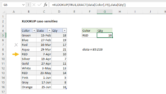
XLOOKUP solution
The XLOOKUP function can be configured to perform a case-sensitive lookup using EXACT in the same way as INDEX and MATCH, but in a more compact formula:
=XLOOKUP(TRUE,EXACT(J5,B5:B14),C5:C14)
Notice the lookup_value and lookup_array are configured like the MATCH function above. After EXACT runs, we have the same array of 10 TRUE and FALSE values explained previously:
=XLOOKUP(TRUE,{FALSE;FALSE;FALSE;FALSE;TRUE;FALSE;FALSE;FALSE;FALSE;FALSE},C5:C14)
XLOOKUP returns the 5th item from the range C5:C14 (39) as a final result.
Note: For a more detailed example of a case-sensitive XLOOKUP formula, see this page.