Summary
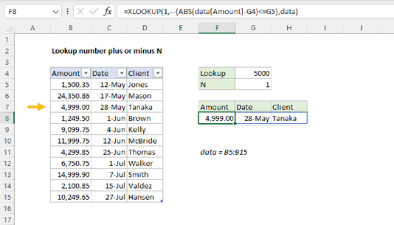
To find the closest match in numeric data, you can use the XLOOKUP function or an INDEX and MATCH formula. In the example shown, the formula in F5 is:
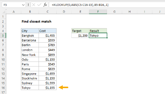
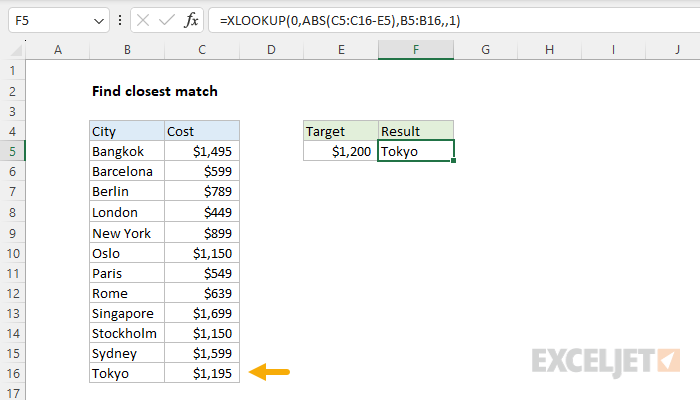
=XLOOKUP(0,ABS(C5:C16-E5),B5:B16,,1)
The result is "Tokyo" because the cost of $1195 is closest to the target value in cell E5, $1200.
Generic formula
=XLOOKUP(0,ABS(values-A1),results,,1)
Explanation
In this example, the goal is to find the closest match to a target value entered in cell E5. Although it may not look like it, this is essentially a look-up problem. The easiest way to solve this problem is with the XLOOKUP function. However in older versions of Excel without the XLOOKUP function, you can use an INDEX and MATCH formula. Both approaches are explained below.
XLOOKUP solution
The XLOOKUP function provides an interesting way to solve this problem because one of XLOOKUP's core features is the ability to perform an approximate match on unsorted data. This sounds very abstract, but we can use this feature to look for a difference of zero between a target value and a set of data, and we don't need to worry about where in the data this match might be. The trick is that we need to calculate the actual differences on-the-fly and use the result as our lookup array. Then we look for a difference of zero. This is the approach used in the workbook shown, where the formula in cell F5 is:
=XLOOKUP(0,ABS(C5:C16-E5),B5:B16,,1)
Notice the lookup_value is zero (0) and the return_array is B5:B16, the range that contains the city names. The clever bit is the lookup_array, which is calculated like this:
ABS(C5:C16-E5)
Working from the inside out, the first operation is to subtract the value in E5 from all costs in C5:C16. Because there are 12 values in C5:C16, this is an array operation, and the result is an array that contains 12 values like this:
ABS({295;-601;-411;-751;-301;-50;-651;-561;499;-50;399;-5})
These values represent the differences between 1200 and the values in C5:C16. Notice many values are negative. To normalize these values, we use the ABS function, which converts the numbers to absolute values. We use the ABS function here because some of the differences are negative, but we only care about absolute differences when looking for the closest match. The result from ABS looks like this:
{295;601;411;751;301;50;651;561;499;50;399;5}
This array is returned directly to the XLOOKUP function as the lookup_array:
=XLOOKUP(0,{295;601;411;751;301;50;651;561;499;50;399;5},B5:B16,,1)
The if_not_found argument is left empty. Finally, we get to the match_mode argument, which is key to the successful operation of the formula. By default, match_mode is zero, which means "exact match". We don't want an exact match in this problem because we are looking for a difference of zero and in most cases, we won't find a perfect match. Instead, the behavior we want is "exact match or next largest value". To enable this behavior, we use the number 1 for match_mode. (More details on XLOOKUP here).
With the configuration explained above, and a target value of $1200 in cell E5, the final result is "Tokyo", because the difference between $1200 and $1195 is $5, and 5 is the closest match to zero. The next closest match is Stockholm, with a cost of $1,150 and a difference of $50.
INDEX and MATCH solution
In older versions of Excel without the XLOOKUP function, you can use an array formula based on INDEX and MATCH like this:
{=INDEX(B5:B16,MATCH(MIN(ABS(C5:C16-E5)),ABS(C5:C16-E5),0))}
Note: this is an array formula and must be entered with control + shift + enter in Excel 2019 and previous.
At the core, this is an INDEX and MATCH formula: MATCH locates the position of the closest match, feeds the position to INDEX, and INDEX returns the value at that position in the range B5:B16. The hard work is done with the MATCH function, which is carefully configured to match the "minimum difference" like this:
MATCH(MIN(ABS(C5:C16-E5)),ABS(C5:C16-E5),0)
Taking things step-by-step, the lookup value in MATCH is calculated with MIN and ABS like this:
MIN(ABS(C5:C16-E5)
First, the value in E5 is subtracted from the values in C5:C16. This is an array operation, and since there are 12 values in the range, the result is an array with 10 values like this:
MIN(ABS({295;-601;-411;-751;-301;-50;-651;-561;499;-50;399;-5}))
These numbers represent the difference between each cost in C5:C16 and the cost in cell E5, 1200. Some values are negative because a cost is lower than the number in E5. To convert negative values to positive values, we use the ABS function, which returns the following array:
MIN({295;601;411;751;301;50;651;561;499;50;399;5}) // returns 5
We are looking for the closest match, so we use the MIN function to find the smallest difference, which is 5. This becomes the lookup value inside MATCH. The lookup array is generated in the same way:
ABS(C5:C16-E5) // generate lookup array
The ABS function then returns the same array we saw above:
{295;601;411;751;301;50;651;561;499;50;399;5}
We now have what we need to find the position of the closest match (smallest difference), and we can rewrite the MATCH portion of the formula like this:
MATCH(5,{295;601;411;751;301;50;651;561;499;50;399;5},0) // returns 12
With 5 as the lookup value, MATCH returns 12, since 5 is in the 12th position in the array:
=INDEX(B5:B16,12)
The INDEX function then returns the 12th city in the range, "Tokyo", as a final result.
Note: if there is a tie, this formula will return the first match.