Summary
To perform a case-sensitive lookup with the SUMPRODUCT function, you can use the EXACT function. In the example, the formula in G5, copied down, is:
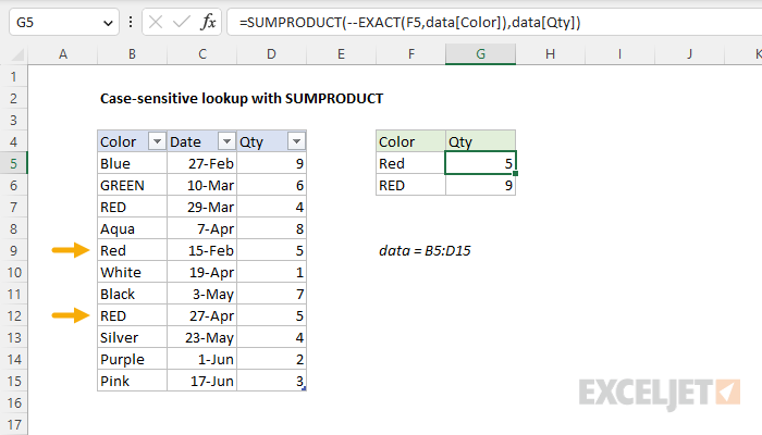
=SUMPRODUCT(--EXACT(F5,data[Color]),data[Qty])
Where "data" is an Excel Table in the range B5:D15. The result is the quantity associated with "Red" (5), excluding "RED". In cell G6, the same formula copied down returns 9, matching "RED". Note that if there is more than one match (i.e. exact match duplicate colors), SUMPRODUCT will sum matching results.
Note: While this is an array formula, it does not need to be entered with Control + Shift + Enter in older versions of Excel, since SUMPRODUCT handles arrays natively. In modern versions of Excel that support dynamic array formulas, there is no advantage to using SUMPRODUCT to solve a problem like this. Instead, switch to XLOOKUP or INDEX and MATCH.
Generic formula
=SUMPRODUCT(--(EXACT(val,lookup_col)),result_col)
Explanation
The SUMPRODUCT function multiplies arrays together and returns the sum of products. If only one array is supplied, SUMPRODUCT will simply sum the items in the array. For example, if we give SUMPRODUCT one array in the form of the data[Qty] column:
=SUMPRODUCT(data[Qty]) // returns 54
SUMPRODUCT returns 54, the total of all numbers in the Qty column, like this:
=SUMPRODUCT(data[Qty])
=SUMPRODUCT({9;6;4;8;5;1;7;5;4;2;3})
=54
What we need now is a way to "filter" these values to include only the value associated with "Red", respecting case. In other words, we need to test the values in the Color column and only allow those associated with "Red" to make it through. We can do this with the EXACT function, which is designed to perform a case-sensitive comparison of text strings. We use EXACT like this:
--EXACT(F5,data[Color])
Because we are comparing the in value in F5 ("Red") with the eleven values in the Color column, the EXACT function returns 11 results in an array like this:
{FALSE;FALSE;FALSE;FALSE;TRUE;FALSE;FALSE;FALSE;FALSE;FALSE;FALSE}
Next, we use a double negative (--) in front of EXACT to convert the TRUE and FALSE values to 1s and 0s. The resulting array looks like this:
{0;0;0;0;1;0;0;0;0;0;0}
Notice the 1 in the 5th position corresponds to the "Red" in row 5. Every other value is now a zero. This will work perfectly as a filter. Turning back to the formula in G5, we can see how this works. The formula is evaluated like this:
=SUMPRODUCT(--EXACT(F5,data[Color]),data[Qty])
=SUMPRODUCT({0;0;0;0;1;0;0;0;0;0;0},{9;6;4;8;5;1;7;5;4;2;3})
=SUMPRODUCT({0;0;0;0;5;0;0;0;0;0;0})
=5
Each array is evaluated, the two arrays are multiplied together, and SUMPRODUCT returns the sum of the products. The FALSE values created with the EXACT function become zeros, and the zeros effectively cancel out the other values when the two arrays are multiplied together. The only values that survive are those associated with TRUE, and the final result is 5.
Remember, this formula only works for numeric values, because SUMPRODUCT doesn't handle text.
Case-sensitive sum
Note that because we are using SUMPRODUCT, this formula comes with a unique twist: if there are multiple matches, SUMPRODUCT will return the sum of those matches. For example, the value in cell F6 is "RED", which appears twice in the Color column. The formula in G6 returns 9 like this:
=SUMPRODUCT(--EXACT(F6,data[Color]),data[Qty])
=SUMPRODUCT({0;0;1;0;0;0;0;1;0;0;0}*{9;6;4;8;5;1;7;5;4;2;3})
=SUMPRODUCT({0;0;4;0;0;0;0;5;0;0;0}) // returns 9
The value "RED" appears in row 3 and row 8 of the table, and the final sum is 9.
Compact syntax
In more advanced SUMPRODUCT formulas, you will often see an abbreviated syntax like this:
=SUMPRODUCT(EXACT(F6,data[Color])*data[Qty])
Notice we are now providing just one array to SUMPRODUCT, which is a result of multiplying the two arrays together directly. The advantage of this approach is that we no longer need to use the double negative. The math operation of multiplying the arrays together automatically coerces the TRUE and FALSE values in the first array into 1s and 0s.