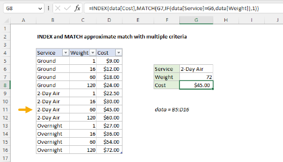
Summary
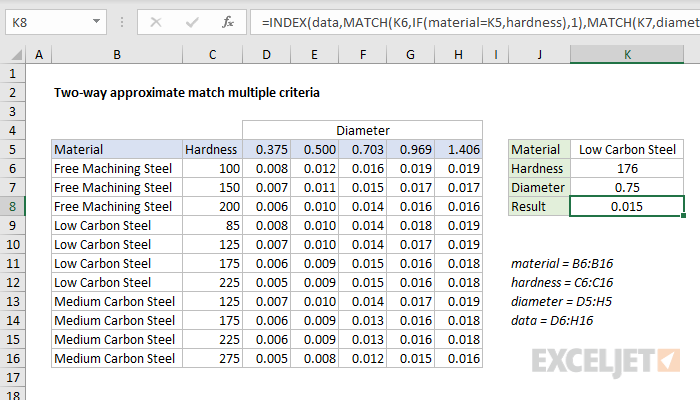
To perform a two-way approximate match lookup with multiple criteria, you can use an array formula based on INDEX and MATCH, with help from the IF function to apply criteria. In the example shown, the formula in K8 is:
=INDEX(data,MATCH(K6,IF(material=K5,hardness),1),MATCH(K7,diameter,1))
where data (D6:H16), diameter (D5:H5), material (B6:B16), and hardness (C6:C16) are named ranges used for convenience only.
Note: this is an array formula and must be entered with Control + Shift + Enter
This is an advanced array formula. If you are new to INDEX and MATCH, start here.
Explanation
The goal is to lookup a feed rate based on material, hardness, and drill bit diameter. Feed rate values are in the named range data (D6:H16).
This can be done with a two-way INDEX and MATCH formula. One MATCH function works out the row number (material and hardness), and the other MATCH function finds the column number (diameter). The INDEX function returns the final result.
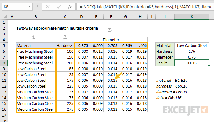
In the example shown, the formula in K8 is:
=INDEX(data,
MATCH(K6,IF(material=K5,hardness),1), // get row
MATCH(K7,diameter,1)) // get column
(Line breaks added for readability only).
The tricky bit is that material and hardness need to be handled together. We need to restrict MATCH to the hardness values for a given material (Low Carbon Steel in the example shown).
We can do this with the IF function. Essentially, we use IF to "throw away" irrelevant values before we look for a match.
Details
The INDEX function is given the named range data (D6:H16) as for array. The first MATCH function works out the row number:
MATCH(K6,IF(material=K5,hardness),1) // get row num
To locate the correct row, we need to do an exact match on material, and an approximate match on hardness. We do this by using the IF function to first filter out irrelevant hardness:
IF(material=K5,hardness) // filter
We test all of the values in material (B6:B16) to see if they match the value in K5 ("Low Carbon Steel"). If so, the hardness value is passed through. If not, IF returns FALSE. The result is an array like this:
{FALSE;FALSE;FALSE;85;125;175;225;FALSE;FALSE;FALSE;FALSE}
Notice the only surviving values are those associated with Low Carbon Steel. The other values are now FALSE. This array is returned directly to the MATCH function as the lookup_array.
The lookup value for match comes from K6, which contains the given hardness, 176. MATCH is configured for approximate match by setting match_type to 1. With these settings, MATCH ignores FALSE values and returns the position of an exact match or the next smallest value.
Note: hardness values must be sorted in ascending order for each material.
With hardness given as 176, MATCH returns 6, delivered directly to INDEX as the row number. We can now rewrite the original formula like this:
=INDEX(data,6,MATCH(K7,diameter,1))
The second MATCH formula finds the correct column number by performing an approximate match on diameter:
MATCH(K7,diameter,1) // get column num
Note: values in diameter D5:H5 must be sorted in ascending order.
The lookup value comes from K7 (0.75), and the lookup_array is the named range diameter (D5:H5).
As before, the MATCH is set to approximate match by setting match_type to 1.
With diameter given as 0.75, MATCH returns 3, delivered directly to the INDEX function as the column number. The original formula now resolves to:
=INDEX(data,6,3) // returns 0.015
INDEX returns a final result of 0.015, the value from F11.