Two-way lookup with INDEX and MATCH

Summary

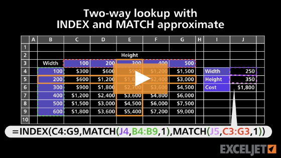
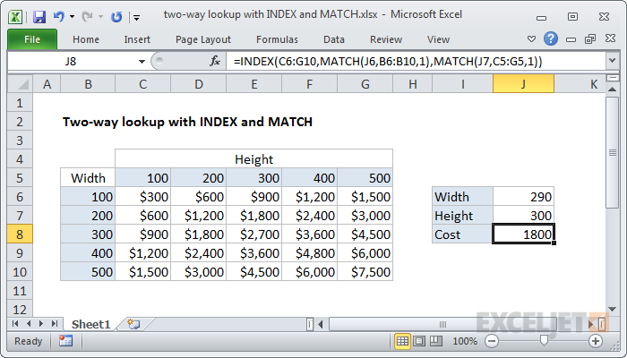
To lookup in value in a table using both rows and columns, you can build a formula that does a two-way lookup with INDEX and MATCH. In the example shown, the formula in J8 is:

=INDEX(C6:G10,MATCH(J6,B6:B10,1),MATCH(J7,C5:G5,1))

Note: this formula is set to "approximate match", so row values and column values must be sorted.

Generic formula

=INDEX(data,MATCH(val,rows,1),MATCH(val,columns,1))

Explanation

The core of this formula is INDEX, which is simply retrieving a value from C6:G10 (the "data") based on a row number and a column number.

=INDEX(C6:G10, row, column)

To get the row and column numbers, we use MATCH, configured for approximate match, by setting the 3rd argument to 1 (TRUE):

MATCH(J6,B6:B10,1) // get row number
MATCH(J7,C5:G5,1) // get column number

In the example, MATCH will return 2 when width is 290, and 3 when height is 300.

In the end, the formula reduces to:

=INDEX(C6:G10, 2, 3)
= 1800

Author

Dave Bruns

Hi - I'm Dave Bruns, and I run Exceljet with my wife, Lisa. Our goal is to help you work faster in Excel. We create short videos, and clear examples of formulas, functions, pivot tables, conditional formatting, and charts.