INDEX and MATCH descending order

To retrieve values from a table where lookup values are sorted in descending order [Z-A] you can use INDEX and MATCH, with MATCH configured for approximate match using a match type of -1. In the example shown, the formula in F5 is:

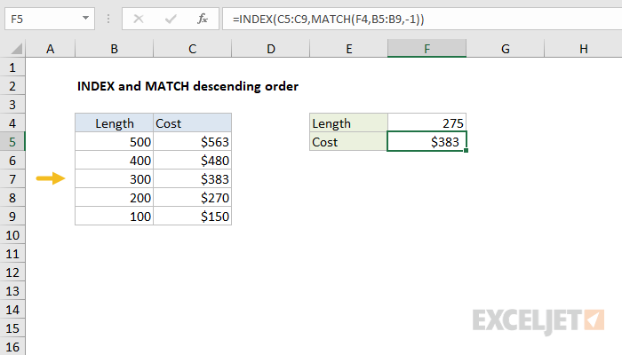
=INDEX(C5:C9,MATCH(F4,B5:B9,-1))

where values in B5:B9 are sorted in descending order.

Context

Suppose you have a product that is sold in rolls of 100 feet, and orders are allowed in whole rolls only. For example, if you need 200 feet of material, you need two rolls total, and if you need 275 feet, you'll need to buy three rolls. In this case, you want the formula to return the "next highest" tier whenever you cross over an even multiple of 100.

Explanation

This formula uses -1 for match type to allow an approximate match on values sorted in descending order. The MATCH part of the formula looks like this:

MATCH(F4,B5:B9,-1)

Using the lookup value in cell F4, MATCH finds the first value in B5:B9 that is greater than or equal to the lookup value. If an exact match is found, MATCH returns the relative row number for that match. When no exact match is found, MATCH continues through the values in B5:B9 until a smaller value is found, then it "steps back" and returns the previous row number.

In the example shown, the lookup value is 275, so MATCH returns a row number of 3 to INDEX: