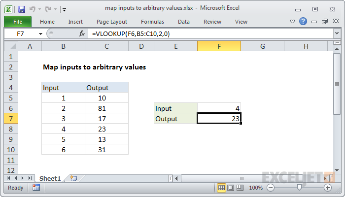
Map inputs to arbitrary values

Summary

If you need to map or translate inputs to arbitrary values, you can use the VLOOKUP function.

In the example, we need to map the numbers 1-6 as follows:

Input	Output
1	10
2	81
3	17
4	23
5	13
6	31

Since there is no way to derive the output (i.e. it's arbitrary), we need to do some kind of lookup. The VLOOKUP function provides an easy way to do this.

In the example shown, the formula in F7 is:

=VLOOKUP(F6,B5:C10,2,0)

Generic formula

=VLOOKUP(input,map_table,column,0)

Explanation

This formula uses the value in cell F6 for a lookup value, the range B5:C10 for the lookup table, 2 to indicate "2nd column", and zero as the last argument to force an exact match.

Although in this case we are mapping numeric inputs to numeric outputs, the same formula will handle text values for both inputs and outputs.

Alternative with CHOOSE

If you have a limited number of inputs, and if the inputs are are numbers starting with 1, you can also use the CHOOSE function. For the example shown the equivalent formula based on CHOOSE is:

=CHOOSE(F6,10,81,17,23,13,31)

The choose function is unwieldy for large amounts of data but for smaller data sets that map to a 1-based index, it has the advantage of being an "all in one" solution.

Author

Dave Bruns

Hi - I'm Dave Bruns, and I run Exceljet with my wife, Lisa. Our goal is to help you work faster in Excel. We create short videos, and clear examples of formulas, functions, pivot tables, conditional formatting, and charts.