Summary
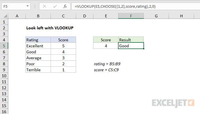
To use VLOOKUP to perform a lookup to the left, you can use the CHOOSE function to reorder the lookup table. In the example shown, the formula in F5 is:
=VLOOKUP(E5,CHOOSE({1,2},score,rating),2,0)
where score (C5:C9) and rating (B5:B9) are named ranges.
Generic formula
=VLOOKUP(A1,CHOOSE({1,2},range2,range1),2,0)
Explanation
One of the VLOOKUP function's key limitations is that it can only look up values to the right. In other words, the column that contains lookup values must sit to the left of the values you want to retrieve with VLOOKUP. There is no way to override this behavior since it is hardwired into the function. As a result, with normal configuration, there is no way to use VLOOKUP to look up a rating in column B based on a score in column C.
One workaround is to restructure the lookup table itself and move the lookup column to the left of the lookup value(s). That's the approach taken in this example, which uses the CHOOSE function reverse rating and score like this:
CHOOSE({1,2},score,rating)
Normally, CHOOSE is used with a single index number as the first argument, and the remaining arguments are the values to choose from. However, here we give choose an array constant for the index number containing two numbers: {1,2}. Essentially, we are asking choose for both the first and second values.
The values are provided as the two named ranges in the example: score and rating. Notice however that we are providing these ranges in reversed order. The CHOOSE function selects both ranges in the order provided and returns the result as a single array like this:
{5,"Excellent";4,"Good";3,"Average";2,"Poor";1,"Terrible"}
CHOOSE returns this array directly to VLOOKUP as the table array argument. In other words, CHOOSE is delivering a lookup table like this to VLOOKUP:
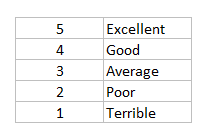
Using the lookup value in E5, VLOOKUP locates a match inside the newly created table and returns a result from the second column.
Reordering with the array constant
In the example shown, we are reordering the lookup table by reversing "rating" and "score" inside the CHOOSE function. However, we could instead use the array constant to reorder like this:
CHOOSE({2,1},rating,score)
The result is exactly the same.
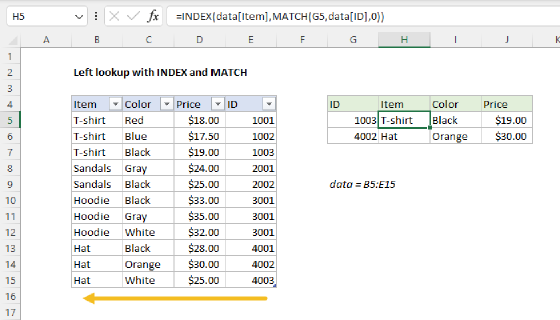
With INDEX and MATCH
While the above example works fine, it isn't ideal. For one thing, most average users won't understand how the formula works. A more natural solution is INDEX and MATCH. Here is the equivalent formula:
=INDEX(rating,MATCH(E5,score,0))
In fact, this is a good example of how INDEX and MATCH is more flexible than VLOOKUP.