Summary
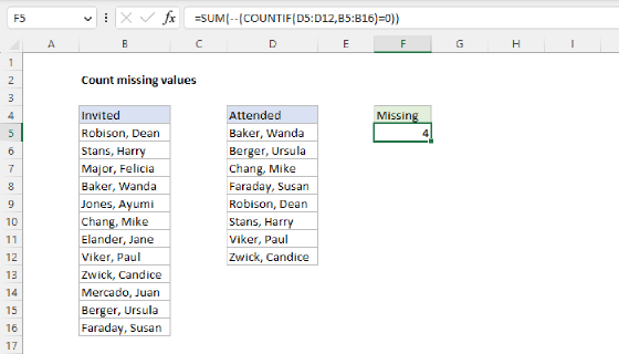
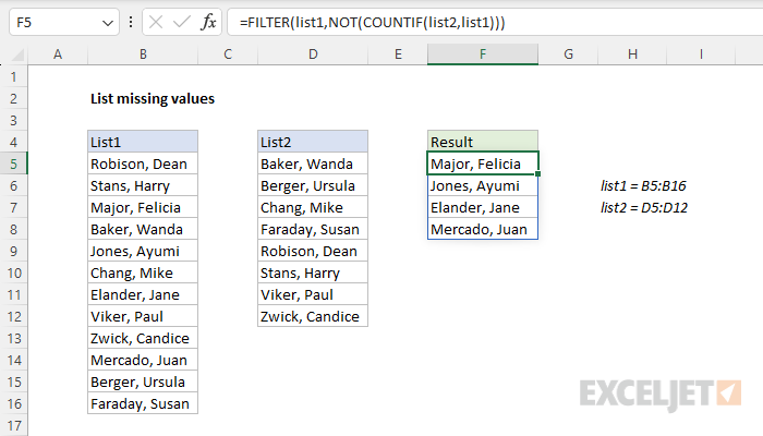
To compare two lists and pull missing values into a new list, you can use the FILTER function. In the example shown, the formula in cell F5 is:
=FILTER(list1,NOT(COUNTIF(list2,list1)))
where list1 (B5:B16) and list2 (D5:D12) are named ranges. The result is the names in B5:B16 that do not appear in D5:D12. See below for an alternative formula based on the XMATCH function that works with arrays as well as ranges.
Generic formula
=FILTER(list1,NOT(COUNTIF(list2,list1)))
Explanation
In this example, the worksheet contains two lists of names. The first list is people who were invited to an event. The second list is people who actually attended the event. For convenience, list1 (B5:B16) and list2 (D5:D12) are named ranges. The goal is to find people who were invited but did not attend the event. That is, we want to list "missing" people as shown in column F.
A good way to solve this problem is with the FILTER function, which is great for finding all matches in a set of data. The twist in this case is that the data itself does not contain the information we need to locate specific names. In other words, there is no field called "Missing" that we can use to filter on. Instead, we need to construct a custom logical test that generates this information.
The article below explains two ways to go about this. The first approach uses COUNTIF + NOT to identify people in list1 who do not appear in list2. This is an intuitive solution that works well, but it does have an important limitation: list2 must be a proper range, not an array. The second approach uses an alternative formula based on the XMATCH function that works with arrays as well as ranges.
FILTER with COUNTIF
This formula uses the FILTER function to retrieve data based on a logical test built with the COUNTIF function. In the worksheet shown, the formula in cell F5 is:
=FILTER(list1,NOT(COUNTIF(list2,list1)))
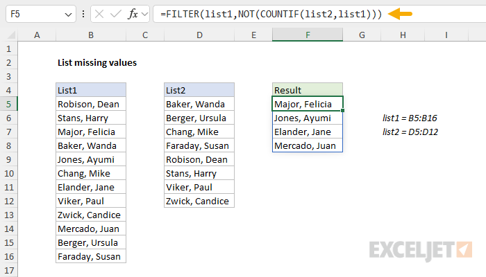
In a nutshell, COUNTIF counts people in list1 who also appear in list2. Then, the NOT function reverses the count to flag the people who are missing. Working from the inside out, the COUNTIF function is used to create the actual filter:
COUNTIF(list2,list1)
Notice we are using list2 as the range argument, and list1 as the criteria argument. In other words, we ask COUNTIF to count all values in list1 that appear in list2. Because we are giving COUNTIF multiple values for the criteria, we get back an array with multiple results:
{1;1;0;1;0;1;0;1;1;0;1;1}
Note that the array contains 12 counts, one for each value in list1. Also, notice that there are 4 zeros in the array. A zero value indicates a name in list1 that was not found in list2. The 1's in the array indicate a name in list1 that was found in list2. Because we want to list names that did not attend, we deliver the result from COUNTIF to the NOT function:
NOT({1;1;0;1;0;1;0;1;1;0;1;1})
The NOT function effectively reverses the result from COUNTIF. Any non-zero number becomes FALSE, and any zero value becomes TRUE. The result from NOT is an array like this:
{FALSE;FALSE;TRUE;FALSE;TRUE;FALSE;TRUE;FALSE;FALSE;TRUE;FALSE;FALSE}
Notice there are now 4 TRUE values in the array. This is what we need to report the missing names. The array is returned directly to the FILTER function as the include argument, and the FILTER function uses the array as a filter. The result is an array of 4 missing names that land in cell F5 and spill into the range F5:F8. If any data changes, FILTER will recalculate and return an updated list.
FILTER with XMATCH
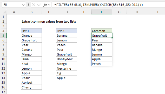
Another way to solve this problem is with a formula that combines the XMATCH function with the ISNA function. In the worksheet below, the formula in cell F5 is:
=FILTER(list1,ISNA(XMATCH(list1,list2)))
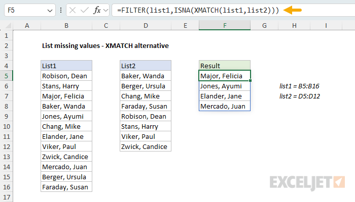
In this formula, we use XMATCH to locate list1 values in list2. Then we reverse the results with the ISNA function. The final result is the same as the original formula: the four names in list1 that do not appear in list2 spill into the range F5:F8. Working from the inside out, XMATCH is configured to look up all values in list1 in list2:
XMATCH(list1,list2)
Because we are giving XMATCH 12 lookup values, we get back an array with 12 results:
{5;6;#N/A;1;#N/A;3;#N/A;7;8;#N/A;2;4}
The numbers in this array record the position of names in list1 that were found in list2. For example, the 5 tells us that "Robison, Dean" appears in the fifth row of list2. The #N/A errors indicate names in list1 that were not found in list2. Since we want the missing names, we hand this result to the ISNA function:
ISNA({5;6;#N/A;1;#N/A;3;#N/A;7;8;#N/A;2;4})
ISNA returns TRUE for #N/A errors and FALSE for everything else, so the result is an array like this:
{FALSE;FALSE;TRUE;FALSE;TRUE;FALSE;TRUE;FALSE;FALSE;TRUE;FALSE;FALSE}
Notice this is exactly the same array created by NOT and COUNTIF in the original formula. As before, the array is returned to the FILTER function as the include argument, and FILTER returns the four missing names, which spill into the range F5:F8.
So why use XMATCH instead of COUNTIF? The main advantage of the XMATCH formula is that it works with arrays as well as ranges. COUNTIF is in a group of eight *IFS functions that won't accept an array for the range argument. This means the original formula will fail if list2 is an array created by another formula. XMATCH does not have this limitation: both lookup_value and lookup_array will accept arrays in memory. If you are working with arrays created by other functions, or if you just want a more universal solution, the XMATCH formula is a better choice. To learn more about how arrays work in Excel formulas, see Arrays in Excel.