NOT Function

The NOT function returns the opposite of a given logical or Boolean value. Use the NOT function to reverse a Boolean value or the result of a logical expression. When given FALSE, NOT returns TRUE. When given TRUE, NOT returns FALSE. The NOT function is commonly used with other functions like IF, AND, and OR to create complex logical tests.

NOT function basics

The purpose of the NOT function is to reverse a Boolean value, for example:

=NOT(TRUE) // returns FALSE
=NOT(FALSE) // returns TRUE

NOT is often used to reverse the result from another function. For example, if cell A1 contains "purple", the formula below will return FALSE since A1 is neither "green" nor "red":

=OR(A1="green",A1="red") // returns FALSE

If we want to reverse this logic, we can wrap the OR function inside the NOT function:

=NOT(OR(A1="green",A1="red")) // returns TRUE

The OR function returns FALSE (as before), and the NOT function returns TRUE. 

Example - NOT this OR that

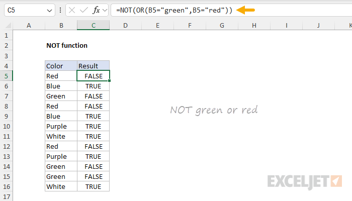
In the worksheet below, the goal is to test each color in column B and return TRUE if the color is not "green" or "red". The formula in C5, copied down, is:

=NOT(OR(B5="green",B5="red"))

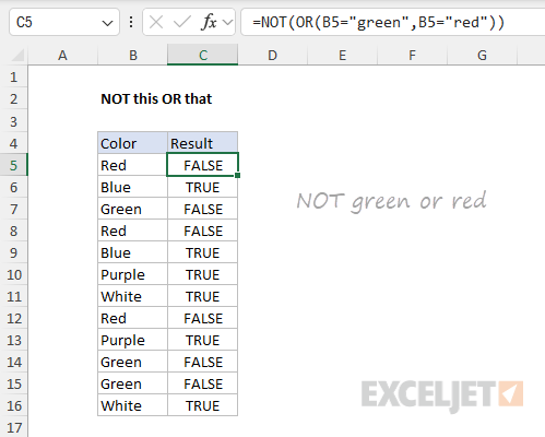
The literal translation of this formula is "NOT green or red". At each row, the formula returns TRUE if the color in column B is not green or red, and FALSE if the color is green or red.

Example - IF + NOT

The NOT function is often used inside the IF function as a logical test. For example, in the worksheet below, the goal is to "flag" colors that are not "red" or "green" with an "x". The formula in cell C5 looks like this:

=IF(NOT(OR(B5="red",B5="green")),"x","")

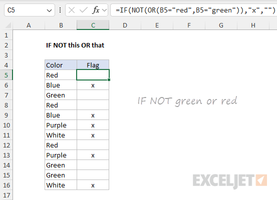
As the formula is copied down, it returns an "x" if the color in column B is NOT "green" or "red". Otherwise, the formula returns an empty string ("").

Example - Not blank

A common use case for the NOT function is to reverse the behavior of another function. For example, If cell A1 is blank (empty), the ISBLANK function will return TRUE:

=ISBLANK(A1)  // TRUE if A1 is empty

To reverse this behavior, wrap the NOT function around the ISBLANK function:

=NOT(ISBLANK(A1))  // TRUE if A1 is NOT empty

By adding NOT the output from ISBLANK is reversed. This formula will return TRUE when A1 is not empty and FALSE when A1 is empty. You might use this kind of test to only run a calculation if there is a value in A1:

=IF(NOT(ISBLANK(A1)),B1/A1,"")

Translation: if A1 is not blank, divide B1 by A1, otherwise return an empty string (""). This is an example of nesting one function inside another.