Highlight column differences

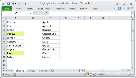
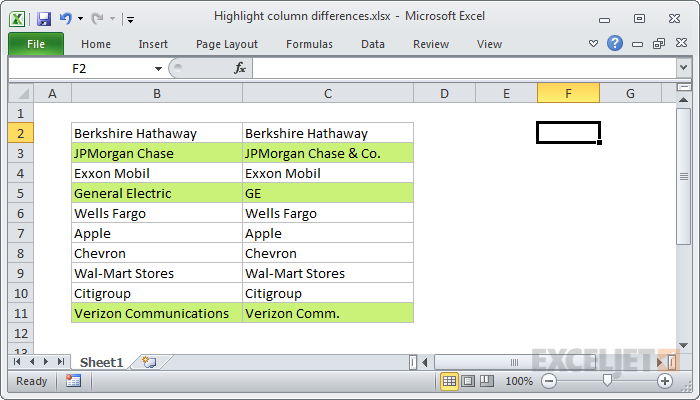
To highlight the differences between two columns of data with conditional formatting you can use a simple formula that uses the "not equal to" operator (e.g. <>) and mixed references. In the example shown, the formula used to highlight differences in the ranges B2:B11 and C2:C11 looks like this:

=$B2<>$C2

Note: with conditional formatting, it's important that the formula be entered relative to the "active cell" in the selection, which is assumed to be B2 in this case.

Explanation

In this example, the goal is to highlight differences in two ranges, B2:B11 and C2:C11, using conditional formatting. To do this, we need to create a new conditional formatting rule, triggered by a formula, like this:

Select the range B2:C11, starting at cell B2.
Select Home > Conditional Formatting > New Rule
Select "Use a formula to determine which cells to format"
Enter the formula =$B2<>$C2 in the input area
Set the desired format to highlight differences
Save the rule

When you use a formula to apply conditional formatting, the formula is evaluated relative to the active cell in the selection at the time the rule is created. In this case, the rule is evaluated for each of the 20 cells in the two columns of data.

The references to $B2 and $C2 are "mixed references" - the column is locked, but the row is relative. This means only the row number will change as the formula is evaluated. Whenever two values in a row are not equal, the formula returns TRUE and the conditional formatting is applied.

A case-sensitive option

Note that the "equals to" (=) and "not equals to" (<>) operators are not case-sensitive. If you need a case-sensitive comparison, you can use the EXACT function with NOT, like so:

=NOT(EXACT($B2,$C2))

EXACT performs a case-sensitive comparison and returns TRUE when values match. The NOT function reverses this logic so that the formula returns TRUE only when the values don't match.

Another approach

One problem with this approach is that if there is an extra or missing value in one column, or if the data is not sorted, many rows will be highlighted as different. Another approach is to count instances that appear in one range but do not appear in another. For details on this approach, see highlight missing values.