Summary
Although Excel ships with many conditional formatting "presets", these are limited. A more powerful way to apply conditional formatting is with formulas, because formulas allow you to apply rules that use more sophisticated logic. This article shows 10 examples, including how to highlight rows, column differences, missing values, and how to build Gantt charts and search boxes with conditional formatting.
Quick Links
Conditional formatting is a fantastic way to quickly visualize data in a spreadsheet. With conditional formatting, you can do things like highlight dates in the next 30 days, flag data entry problems, highlight rows that contain top customers, show duplicates, and more.
Excel ships with a large number of "presets" that make it easy to create new rules without formulas. However, you can also create rules with your own custom formulas. By using your own formula, you take over the condition that triggers a rule and can apply exactly the logic you need. Formulas give you maximum power and flexibility.
For example, using the "Equal to" preset, it's easy to highlight cells equal to "apple".
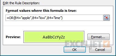
But what if you want to highlight cells equal to "apple" or "kiwi" or "lime"? Sure, you can create a rule for each value, but that's a lot of trouble. Instead, you can simply use one rule based on a formula with the OR function:
Here's the result of the rule applied to the range B4:F8 in this spreadsheet:
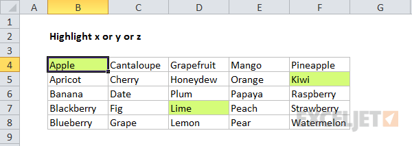
Here's the exact formula used:
=OR(B4="apple",B4="kiwi",B4="lime")
Quick start
You can create a formula-based conditional formatting rule in four easy steps:
- Select the cells you want to format.
- Create a conditional formatting rule, and select the Formula option
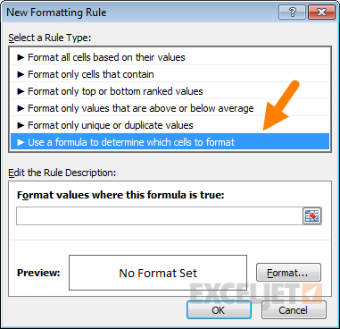
- Enter a formula that returns TRUE or FALSE.
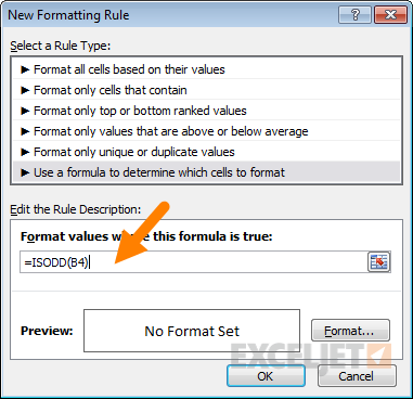
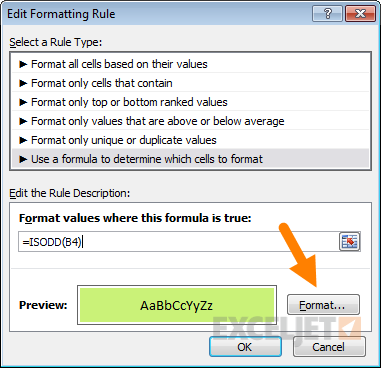
- Set formatting options and save the rule.
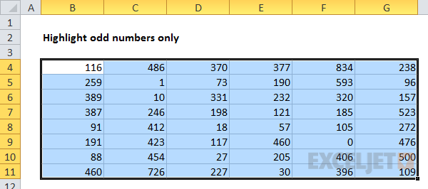
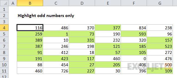
The ISODD function only returns TRUE for odd numbers, triggering the rule:
Video: How to apply conditional formatting with a formula
We also offer video training on conditional formatting.
Formula logic
Formulas that apply conditional formatting must return TRUE or FALSE, or numeric equivalents. Here are some examples:
=ISODD(A1)
=ISNUMBER(A1)
=A1>100
=AND(A1>100,B1<50)
=OR(F1="MN",F1="WI")
The above formulas all return TRUE or FALSE, so they work perfectly as a trigger for conditional formatting.
When conditional formatting is applied to a range of cells, enter cell references with respect to the upper-left cell. The trick to understanding how conditional formatting formulas work is to visualize the same formula being applied to each cell in the selection, with cell references updated as usual. Imagine that you entered the formula in the upper-left cell of the selection, and then copied the formula across the entire selection. If you struggle with this, see the section on Dummy Formulas below.
Formula Examples
Below are examples of custom formulas you can use to apply conditional formatting. Some of these examples can be created using Excel's built-in presets for highlighting cells, but custom formulas can go far beyond presets, as you can see below.
Highlight orders from Texas
To highlight rows that represent orders from Texas (abbreviated TX), use a formula that locks the reference to column F:
=$F5="TX"
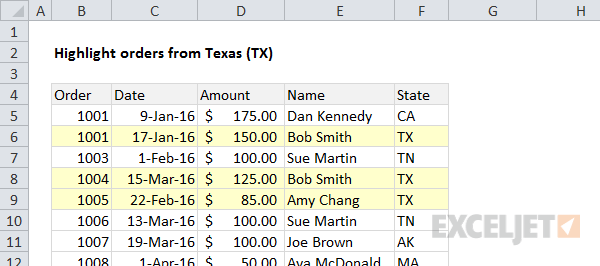
For more details, see this article: Highlight rows with conditional formatting.
Video: How to highlight rows with conditional formatting
Highlight dates in the next 30 days
To highlight dates occurring in the next 30 days, we need a formula that (1) makes sure dates are in the future and (2) makes sure dates are 30 days or less from today. One way to do this is to use the AND function together with the NOW function like this:
=AND(B4>NOW(),B4<=(NOW()+30))
With a current date of August 18, 2016, the conditional formatting highlights dates as follows:
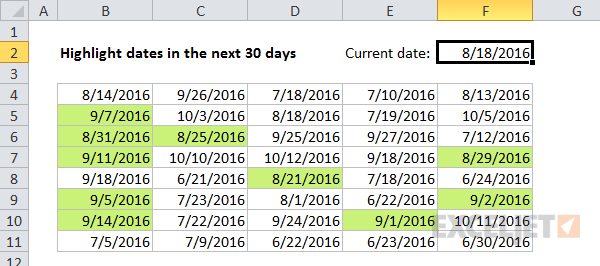
The NOW function returns the current date and time. For details about how this formula, works, see this article: Highlight dates in the next N days.
Highlight column differences
Given two columns that contain similar information, you can use conditional formatting to spot subtle differences. The formula used to trigger the formatting below is:
=$B4<>$C4
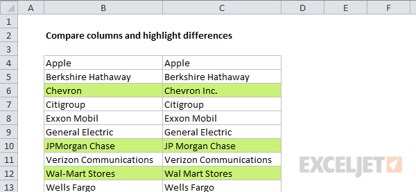
See also: a version of this formula that uses the EXACT function to do a case-sensitive comparison.
Highlight missing values
To highlight values in one list that are missing from another, you can use a formula based on the COUNTIF function:
=COUNTIF(list,B5)=0
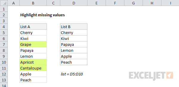
This formula simply checks each value in List A against values in the named range "list" (D5:D10). When the count is zero, the formula returns TRUE and triggers the rule, which highlights values in List A that are missing from List B.
Video: How to find missing values with COUNTIF
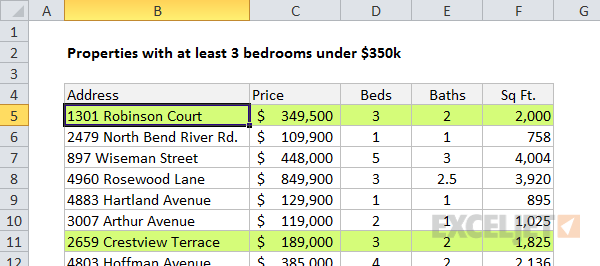
Highlight properties with 3+ bedrooms under $350k
To find properties in this list that have at least 3 bedrooms but are less than $300,000, you can use a formula based on the AND function:
=AND($C5<350000,$D5>=3)
The dollar signs ($) lock the reference to columns C and D, and the AND function is used to make sure both conditions are TRUE. In rows where the AND function returns TRUE, the conditional formatting is applied:
Highlight top values (dynamic example)
Although Excel has presets for "top values", this example shows how to do the same thing with a formula, and how formulas can be more flexible. By using a formula, we can make the worksheet interactive — when the value in F2 is updated, the rule instantly responds and highlights new values.
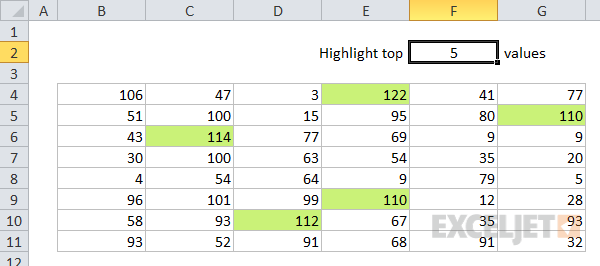
The formula used for this rule is:
=B4>=LARGE(data,input)
Where "data" is the named range B4:G11, and "input" is the named range F2. This page has details and a full explanation.
Gantt charts
Believe it or not, you can even use formulas to create simple Gantt charts with conditional formatting like this:
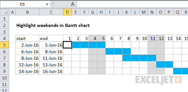
This worksheet uses two rules, one for the bars, and one for the weekend shading:
=AND(D$4>=$B5,D$4<=$C5) // bars
=WEEKDAY(D$4,2)>5 // weekends
This article explains the formula for bars, and this article explains the formula for weekend shading.
Simple search box
One cool trick you can do with conditional formatting is to build a simple search box. In this example, a rule highlights cells in column B that contain text typed in cell F2:
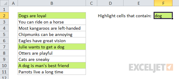
The formula used is:
=ISNUMBER(SEARCH($F$2,B2))
For more details and a full explanation, see:
- Article: How to highlight cells that contain specific text
- Article: How to highlight rows that contain specific text
- Video: How to build a search box to highlight data
Troubleshooting
If you can't get your conditional formatting rules to fire correctly, there's most likely a problem with your formula. First, make sure you started the formula with an equals sign (=). If you forget this step, Excel will silently convert your entire formula to text, rendering it useless. To fix, just remove the double quotes Excel added at either side and make sure the formula begins with equals (=).
If your formula is entered correctly but is not triggering the rule, you may have to dig a little deeper. Normally, you can use the F9 key to check results in a formula or use the Evaluate feature to step through a formula. Unfortunately, you can't use these tools with conditional formatting formulas, but you can use a technique called "dummy formulas".
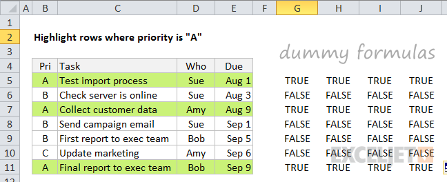
Dummy Formulas
Dummy formulas are a way to test your conditional formatting formulas directly on the worksheet, so you can see what they're actually doing. This can be a big time-saver when you're struggling to get cell references working correctly.
In a nutshell, you enter the same formula across a range of cells that matches the shape of your data. This lets you see the values returned by each formula, and it's a great way to visualize and understand how formula-based conditional formatting works. For a detailed explanation, see this article.
Video: Test conditional formatting with dummy formulas
Limitations
There are some limitations that come with formula-based conditional formatting:
- You can't apply icons, color scales, or data bars with a custom formula. You are limited to standard cell formatting, including number formats, font, fill color, and border options.
- You can't use certain formula constructs like unions, intersections, or array constants for conditional formatting criteria.
- You can't reference other workbooks in a conditional formatting formula.
You can sometimes work around #2 and #3. You may be able to move the logic of the formula into a cell in the worksheet, and then refer to that cell in the formula instead. If you are trying to use an array constant, try creating a named range instead.


