Gantt chart with weekends

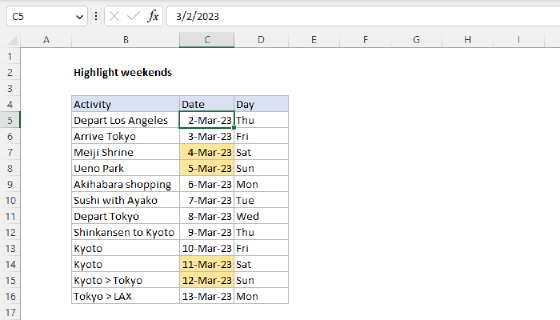
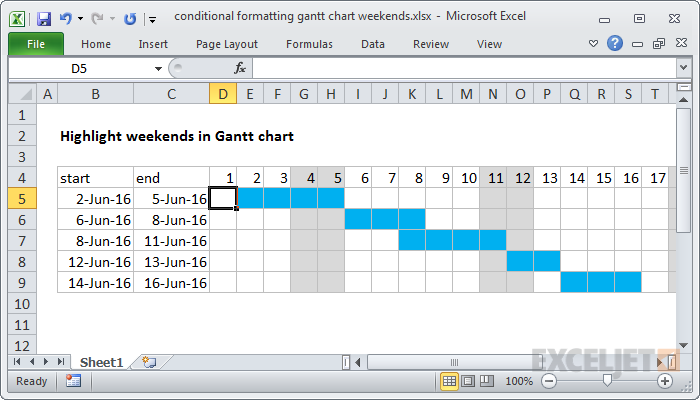
To build a Gantt chart with weekends shaded, you can use Conditional Formatting with a formula based on the weekday function.In the example shown, the formula applied the calendar, starting at D4, is:

=WEEKDAY(D$4,2)>5

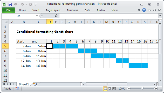
Note: this formula deals with weekend shading only. To see how to build the date bars with conditional formatting, see this article.

Explanation

The key to this approach is the calendar header (row 4), which is just a series of valid dates, formatted with the custom number format "d". With a hardcoded date in D4, you can use =D4+1 to populate the calendar. This allows you to set up a conditional formatting rule that compares the date in row 4 with the dates in columns B and C.

To shade days that are weekends, we are using a formula based on the weekday function. By default, the weekday function returns a number between 1 and 7 that corresponds to days of the week, where Sunday is 1 and Saturday is 7. However, by adding the optional second argument called "return type" with a value of 2, the numbering scheme changes so that Monday is 1 and Saturday and Sunday are 6 and 7, respectively.

As a result, to return TRUE for dates that are either Saturday or Sunday, we only need to test for numbers greater than 5. The conditional formatting formula applied to the calendar area (starting with D4) looks like this:

=WEEKDAY(D$4,2)>5

The reference to D4 is mixed, with the row locked so that the formula continues to evaluate the dates in the header for all rows in the calendar grid.