Summary
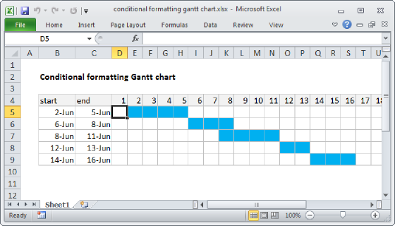
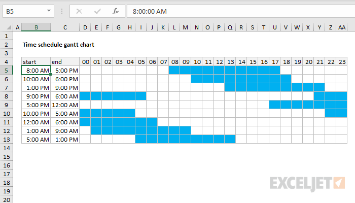
To build a Gantt chart to show a time schedule, you can use Conditional Formatting with a formula based on AND and OR functions. In the example shown, the formula applied to D5 is:
=IF($B5<$C5,AND(D$4>=$B5,D$4<=$C5),OR(D$4>=$B5,D$4<$C5))
Note references are mixed to lock rows and columns as needed in order to test each cell in the grid correctly.
Generic formula
=IF(start<end,AND(A$1>=start,time<=end),OR(A$1>=start,A$1<end))
Explanation
Note: this is a great example of a formula that is hard to understand because the cell references are hard to interpret. The gist of the logic used is this: if the time in row 4 is between the start and end times, the formula should return TRUE and trigger the blue fill via conditional formatting. The actual implementation is a little more complicated because the formula below also takes into account the possibility that the start and end times cross midnight. If this is relevant to your situation, you can use just the AND expression explained below.
The calendar header (row 4) is a series of valid Excel times, formatted with the custom number format "hh". This makes it possible to set up a conditional formatting rule that compares the time associated with each column in row 4 with the times entered in columns B and C.
Each time in row 4 needs to be checked to see if it falls within the start and end times in columns B and C, for each row of data in the schedule. The logic used to apply conditional formatting depends on the start and end times. When the start time is less than the end time (normal case) the AND function is used to trigger conditional formatting. When the start time is greater than the end time (times cross midnight) the OR function is used instead.
To handle this distinction at a high level, the IF function is used first to check each pair of times:
=IF($B5<$C5
When the start time is earlier than the end time, the test above returns TRUE, and IF returns the AND part of the formula:
AND(D$4>=$B5,D$4<=$C5)
The AND function is configured with two conditions. The first condition checks to see if the column time is greater than or equal to the start time:
D$4>=$B5
The second condition checks that the column time is less than or equal to the end time:
D$4<=$C5
When both conditions return TRUE, the formula returns TRUE, and triggers the blue fill for the cells in the calendar grid.
When the start time is greater than the end time (times cross midnight), IF returns an expression constructed with OR:
OR(D$4>=$B5,D$4<$C5)
Here, the OR function is configured with two conditions. The first condition is the same as that used in AND above – it checks to see if the column time is greater than or equal to the start time:
D$4>=$B5
The second condition is altered slightly to check if the column time is less than the end time:
D$4<$C5
When either condition returns TRUE, OR returns TRUE, and triggers the conditional formatting.
Note: both conditions use mixed references to ensure that the references update correctly as conditional formatting is applied to the grid.