Test conditional formatting with dummy formulas

If you've ever applied conditional formatting with your own formula, you know the hardest part is making sure the formula actually works.

The problem is that the formula area in a conditional formatting rule isn't very friendly. You don't get highlighted cell references, you don't get function autocomplete...heck....you don't even get screen tips.

As a result, it's hard to "see" if a formula is going to work until after you save the rule. If it doesn't, you have to use trial and error:

1. Edit the rule
2. Edit the formula using your "best guess"
3. Save the rule to see what happens
4. Repeat as needed

This isn't much fun, and it can be really frustrating when you run into a tricky problem.

Luckily, there's an easy fix: dummy formulas.

A better way - test with dummy formulas

With more complicated conditional formatting formulas, the key is to test the rule with "dummy" formulas first, before you create the rule. This may at first seem impossible — how can you test a conditional formatting formula without applying a conditional format?

The trick is understanding that you can think of conditional formatting as an "overlay" of invisible formulas that sit on top of the cells. When a formula in the overlay returns TRUE for a given cell, the formatting is applied.

So, to test a conditional formatting rule, you just need to build a set of "dummy" formulas on the worksheet that simulates the overlay.

I like to put the test formulas over to the side of the data, lined up with the rows. This makes it easy to set up and match references.

Then, simply write the first formula by referencing the upper left cell in the data. This will be the active cell when the conditional formatting rule is created.

Example 1 - Simple Formula

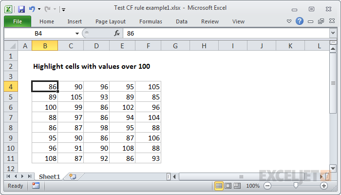
For example, say you have numbers in a table, and you want to highlight values over 100.

Note: Excel contains a conditional formatting "preset" that will highlight values "greater than", so it's not necessary to use a formula to do this. We are just using a basic formula as an example.

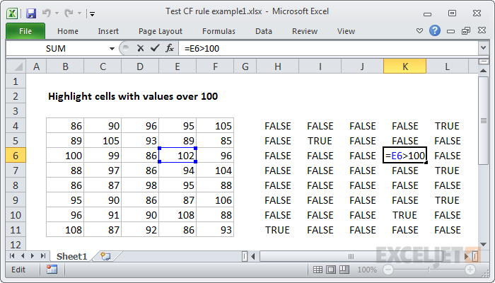
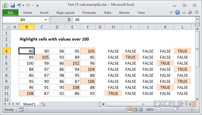
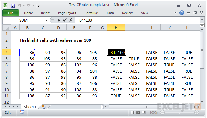
We have plenty of space to the right, so we'll add our dummy formulas there. In cell H4, add the first formula. In this case, we want to use:

=B4>100

Why B4? Because B4 corresponds to the active cell we'll have when we define the actual conditional formatting rule.

Now copy the formula across and down. You only need to copy down as many rows as you want to test. In this case, with a small set of data, we can easily test all rows.

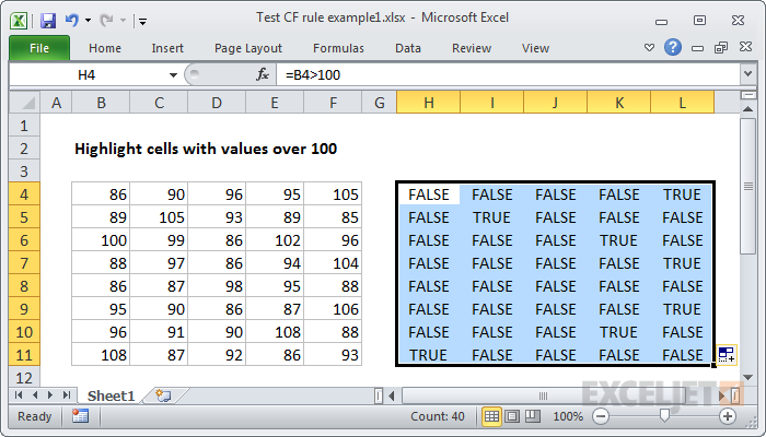
Notice we get a TRUE or FALSE value in every cell. If we check a few references, you can see that each formula is evaluating a cell in the data, relative to B4. All references to B4 have changed, since B4 was entered as a relative address.

Checking references - each formula refers to a cell relative to B4

Now simply imagine these results transposed directly on top of the data. Wherever you see a TRUE value, the conditional formatting will be applied:

Notice that TRUE values are correctly marking the values > 100 in the data (manually highlighted)

The dummy formula looks good, so let's try it out in a conditional formatting rule.

First, copy the formula in the upper left cell of the dummy formulas – that's H4 in this case.

Next, select the data and define a new conditional formatting rule.

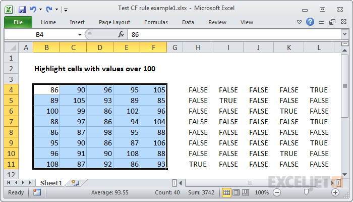
Data selected - note the active cell is B4

Paste the formula into the box, and set the format.

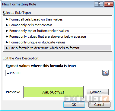
Ready to save the new rule

Success! All cells with values over 100 highlighted:

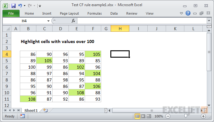
Final conditional formatting applied with a formula, with dummy formulas removed.

Example 2 - a more complicated formula

That was a simple example, so let's try the same approach with a more complicated formula.

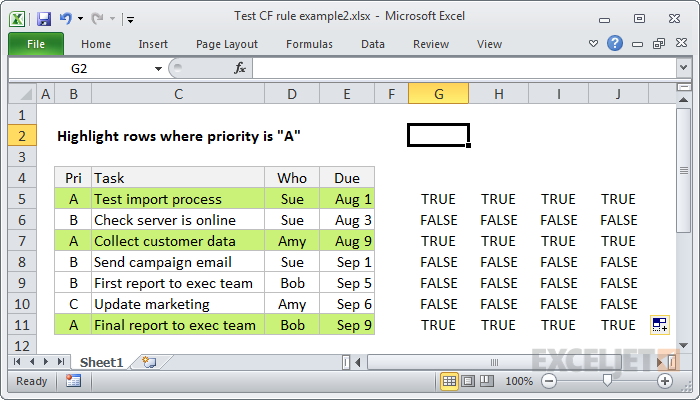
Let's create a rule that highlights rows in a table based on the value in one column. In this case, we'll highlight tasks with a priority of "A".

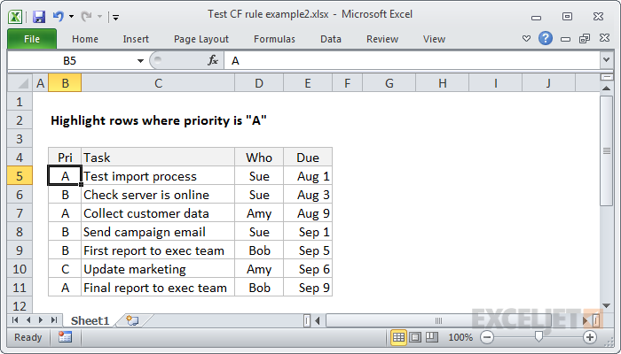
Need to highlight all rows with a priority of "A"

This is a classic problem in conditional formatting. The formula will require a mixed reference, but mixed references can be hard to understand when you aren't able to see references on the worksheet. However, by using dummy formulas, we can easily test and perfect a rule.

As before, the first step is to figure out where to put the test formulas. We have plenty of room to the right, so we'll start in cell G5.

Since we want to highlight tasks with a priority of "A", we'll use this formula to start:

=B5="A"

After I copy the formulas across and down, this is what we have:

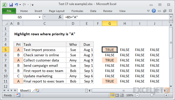
Not going to work - only values in column B will be highlighted (orange shading manually applied)

Notice that we are getting a result of TRUE where the priority is "A", but only for values in column B. It's a good start, but it will only highlight cells in the first column.

We need to adjust the formula so that it returns TRUE for the entire row. To do this, we need to use a mixed reference in the formula to lock the column. The revised formula is:

=$B5="A"

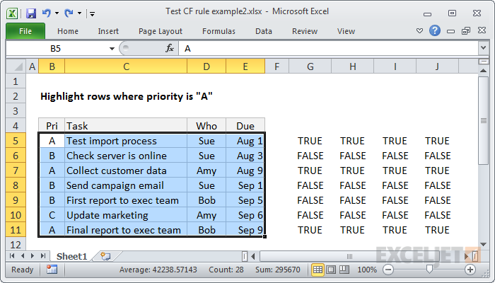
When I copy this new formula across our test range, we get what we need:

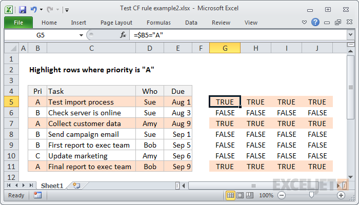
With the column locked, we get an entire row of TRUE's when the priority is "A" (orange shading manually applied)

See how the dummy formulas will work? Imagine them as an overlay on the data itself.

Now let's created the conditional formatting rule. First, select the data:

Data selected, and ready to create new rule (note active cell is B5)

Finally, let's create the rule, using the formula in the upper left:

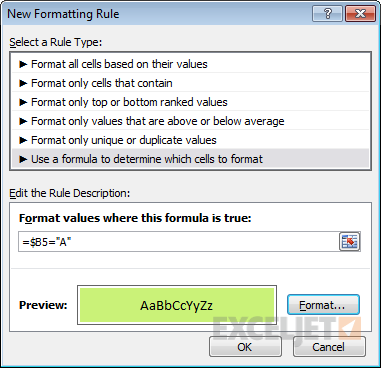
Formula pasted from G5

As you can see, the new rule works perfectly the first time.

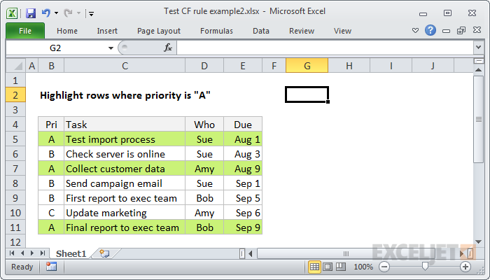
Conditional formatting working as expected (dummy formulas removed)

Conclusion

The next time you need to apply conditional formatting with a more complicated formula, set up dummy formulas next to the data, and fine tune the formula until you get TRUE values where you need them. By working directly on the worksheet, you have full access to all of Excel's formula tools, and you can easily troubleshoot and adjust the formula until it works perfectly.