
Summary
How do you figure out what formula to use? A teardown of 5 good formulas you can use to highlight dates based on a common month and year value using conditional formatting.
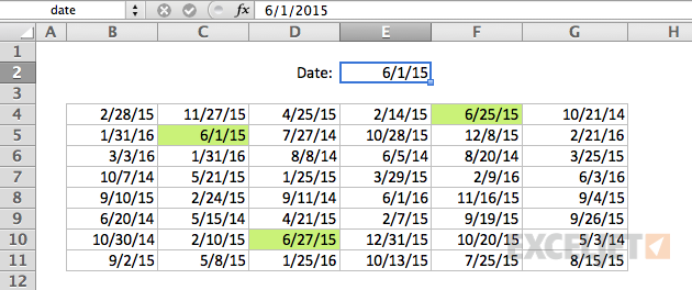
A few days ago, I posted this conditional formatting puzzle:
Given a date, what formula will highlight other dates in the same month and year?
We received some clever formulas as comments, so I want to do a quick teardown of five formulas, and provide a little commentary on each.
Here's the list:
Option #1 - Extract with MONTH and YEAR and test with AND
Option #2 - force dates to first of month and compare
Option #3 - force dates to last of month and compare
Option #4 - concatenate year and month and compare
Option #5 - concatenate year and month with TEXT and compare
Download the practice worksheet attached below and try them out yourself. In the worksheet, cell E2 is named "date".
If you need a quick recap on how to use a formula with conditional formatting, see: How to apply conditional formatting with a formula. Here is another article on Conditional formatting based on a different cell.
The purpose of these formulas is to automatically highlight dates in the table whenever the date in E2 changes.
Option #1 - Extract with MONTH and YEAR and test with AND
The "obvious" solution (if you're an Excel nerd :)) is one that uses the AND function along with MONTH and YEAR. It looks like this:
=AND(YEAR(B4)=YEAR(date),MONTH(B4)=MONTH(date))
This formula uses the AND function to test two conditions:
YEAR(B4)=YEAR(date) // is the year the same?
MONTH(B4)=MONTH(date) // is the month the same?
Both of these conditions use the equal sign to force a TRUE or FALSE result. If both return TRUE, AND returns TRUE and the conditional formatting is triggered.
Pros - intuitive, straightforward
Cons - requires five function calls and four references
I also like this formula because it builds on simple functions that you absolutely need to know: MONTH, YEAR & AND.
Option #2 - force dates to first of month and compare
Another interesting solution is to pull out the month and year from each date and use these values to build "first of the month" dates, which are then compared. The formula looks like this:
=DATE(YEAR(B4),MONTH(B4),1)=DATE(YEAR(date),MONTH(date),1)
There are two main parts of the formula. On the left of the equal sign, the formula extracts the year and month values from B4, then uses those values to create a new date with the day value hard-coded as 1. On the right, the same thing happens with the date in date ($E$2).
=DATE(YEAR(B4),MONTH(B4),1)=DATE(YEAR(date),MONTH(date),1)
=DATE(2015,2,1)=DATE(2015,6,1)
=42036=42156*
=FALSE
- 42036 is the date serial number for 1-Feb-2015 and 42156 is the serial number for 1-Jun-2015, which is how Excel evaluates the dates internally.
In each case, the year and month values are extracted, and used to create a new date where the day value is hard-coded as 1. Effectively, this ignores day completely by making it the same for each date.
Finally, the two dates are tested for equality.
Pros - fairly intuitive
Cons - requires six function calls and four references
What I like about this formula is the creative thinking — the "trick" of forcing the day to 1. You'll find these kind of tricks are everywhere in more complex Excel formulas.
Option #3 - force dates to last of month and compare
Similar to option #3, another clever idea from reader Eric Kalin is to force dates to "last of month" and compare. This is a nice solution because Excel has a dedicated function for getting the last day a month: EOMONTH. The formula looks like this:
=EOMONTH(B4,0)=EOMONTH(date,0)
This formula can be summarized like this: get the last of month using the date in B4 and compare it to the last day of month based on the date in $E$2.
Pros - compact and economical; just two function calls and two references
Cons - need to know and understand EOMONTH
Overall, a very nice formula that stands out for its simplicity.
Option #4 - concatenate year and month and compare
Yet another approach is to extract and concatenate the year and month values for each date, then compare the result:
=MONTH(B4)&YEAR(B4)=MONTH(date)&YEAR(date)
This may not be a solution you'd think of initially, because the idea of concatenating numbers is a little weird.
If you concatenate, say, 11 (November) with the year 2015, you'll get "112015", which is likely not a value you'd recognize at first glance. However, to Excel, it's just a string (text value), and Excel will be happy to compare it with any other string for you. So, here's what the formula looks like for cell B4 and cell $E$2 as it's solved:
=MONTH(B4)&YEAR(B4)=MONTH(date)&YEAR(date)
="22015"="62015"
=FALSE
Pros - logical and relatively compact (4 function calls)
Cons - need to know about concatenation
Option #5 - concatenate year and month with TEXT and compare
Finally, here is another formula that relies on the idea of concatenating the month and year together. However, this formula uses the TEXT function and a custom number format, rather than concatenating manually with the ampersand (&) operator:
=TEXT(B4,"myyyy")=TEXT(date,"myyyy")
TEXT is a useful function that allows you to convert a number to text in the text format of your choice. In this case the format is the custom date format "myyyy", which translates to: month number without leading zeros & 4-digit year.
Like #4 above, the result is the same as concatenating the month and year manually. Solving with B4 and date ($E$2):
=TEXT(B4,"myyyy")=TEXT(date,"myyyy")
="22015"="62015"
=FALSE
Pros - simple and compact (2 function calls)
Cons - need to understand TEXT
What's the best option?
Well, in many cases, the best option is the one you know :)
If you spend a lot of time with Excel formulas, you'll notice an obsession (in yourself, and in others) with compact and elegant formulas. It's hard not to be delighted by a clever and efficient formula. And it's true that shorter formulas offer less chance of making a mistake, since you aren't wrangling as many parentheses and references.
But all that said, Excel is a vehicle, not a destination. Unless you build models professionally, or analyze huge data sets (where efficiency really counts), your boss probably doesn't care what formula you use as long as it gets the job done accurately, and is straightforward to understand.
What's your favorite option? Leave a comment below.
Are you looking for more conditional formatting formulas?


