
Summary
In this article, we look at some cool ways that you can use Excel's conditional formatting feature to quickly visualize important data.
You've heard of data visualization, right? It's the art and science of presenting data in a way so that people can "see" important information at a glance. Data visualization makes complex data more accessible and useful. In a world overflowing with data, it's more valuable than ever.
Excel has a great tool for visualizing data called Conditional Formatting. If you work with data in Excel (and who doesn't these days?) you'll find it incredibly useful. By creating simple rules that highlight just the data you are interested in, you can spot key information very quickly.
To help get you started, and to give you some inspiration, here are some cool ways that you can use Excel conditional formatting to help you understand data faster.
Highlight duplicate or unique values
One of the handy ways you can use conditional formatting is to highlight duplicate or unique values quickly. Excel contains built-in rules to make both of these tasks easy.
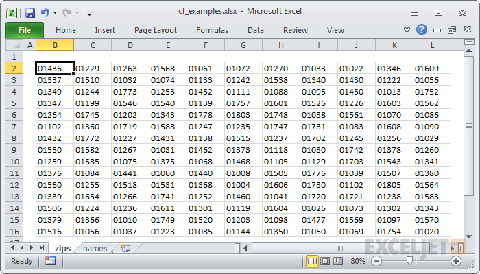
For example, suppose you have this table of zip codes, and you want to highlight duplicate zip codes? With over 160 zip codes in the list, it's almost impossible for the human eye to spot duplicate codes.
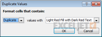
But using Conditional Formatting, you can just select the table and tell Excel to highlight duplicates using a built-in conditional formatting rule for duplicates:
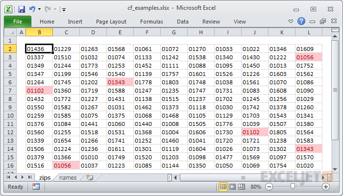
With just a few clicks, here is the result:
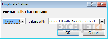
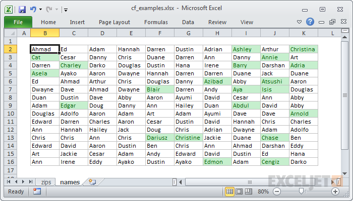
Alternately, suppose you have this table of names and you need to find only unique values (values that appear once)?
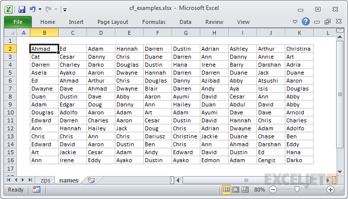
Good luck finding names that appear only once with just your eyes! However, using a built-in conditional formatting rule, you can find all unique names in less than 10 seconds:
Flipping the problem yet again, what if you wanted to find all names that appear at least 5 times? By creating a rule based on a formula:
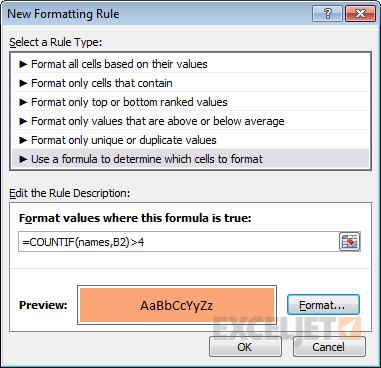
You can easily highlight names that appear at least 5 times:
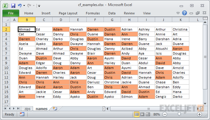
The formula I'm using, with a named range "names" for all names, is this:
=COUNTIF(names,B2)>4
Highlight top or bottom values
Suppose you have the following report, which shows monthly sales totals for the salespeople in your company:
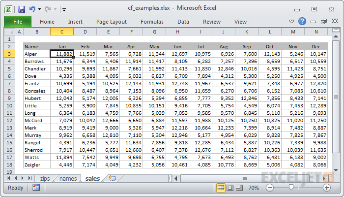
It's nice to have all the information in one place, but you'd like to quickly see the 5 top and 5 bottom sales numbers, so you know where to focus your attention.
By using two built-in conditional formatting rules:
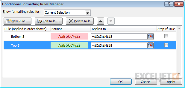
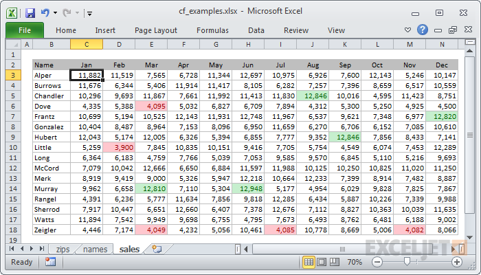
You can flag the top 5 values in green, and the bottom 5 values in red:
Want to learn more? See our video course on conditional formatting.
Highlighting values based on a variable input
Although Excel contains a large number of Conditional Formatting presets, the real power of Conditional Formatting comes from using formulas. Formulas allow you to create more powerful and flexible rules.
For example, suppose you want to explore a data set and highlight values above a certain value, in this case, 800?
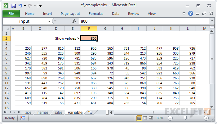
By creating an input cell and referring to that input cell in a formula, you can make the threshold a variable.
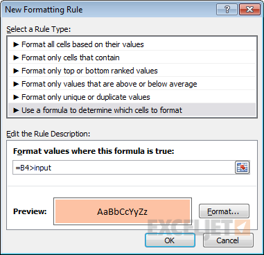
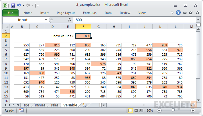
Here the rule highlights all values greater than 800:
Here we've changed the input to 900, highlighting fewer values:
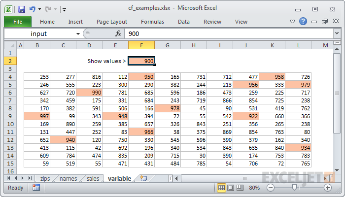
By making the rule variable, you create a model that lets you interactively explore the data. This is a great way to add some professional polish to a worksheet, because people love things that respond instantly to their actions.
Highlight entire rows based on values in a column
There are many situations where you may want to highlight an entire row based on a value that appears in one column. To do this with conditional formatting, you'll need to use a formula and then lock the column reference as needed.
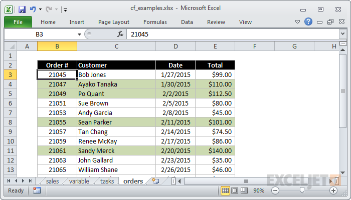
For example, let's say you want to highlight orders in this set of data that are over $100:
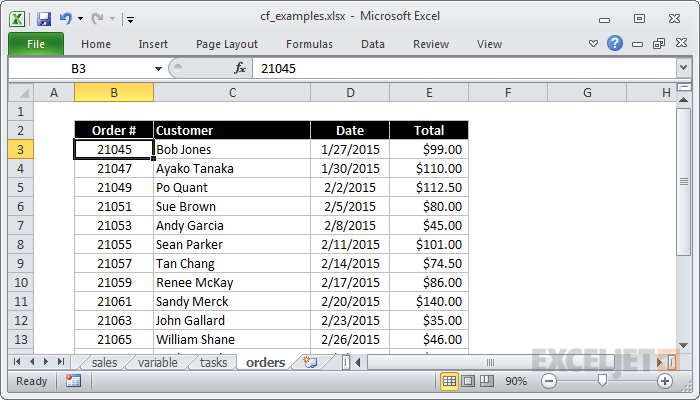
The formula locks the column reference to test only values in column E:
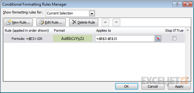
The result:
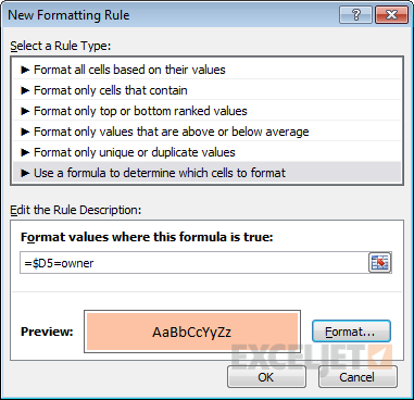
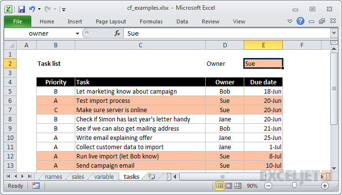
Highlight rows based on an input cell
Building on the previous examples, here we are highlighting rows based on the value in an input cell named "owner".
Build a search box
Using the same basic idea in the last example, you can actually build a search box using conditional formatting that searches multiple columns at the same time. This is a nice alternative to filtering because no data is hidden.
Video: How to build a search box with conditional formatting


