Dynamic calendar grid

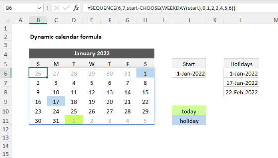
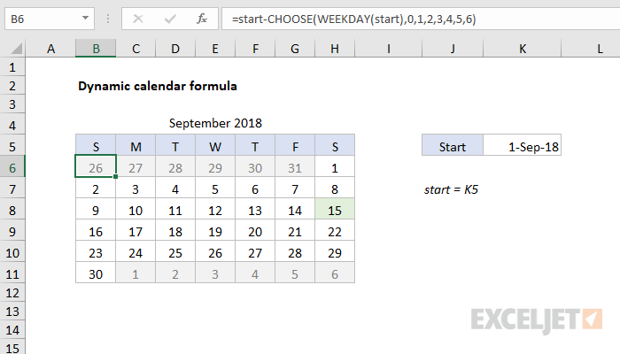
You can set up dynamic calendar grid on an Excel worksheet with a series of formulas, as explained in this article. In the example shown, the formula in B6 is:

=start-CHOOSE(WEEKDAY(start),0,1,2,3,4,5,6)

where "start" is the named range K5, and contains the date September 1, 2018.

Note: this example uses a formula technique that will work in older versions of Excel. For a more modern solution based on the SEQUENCE function, see this example.

Explanation

Note: This example assumes the start date will be provided as the first of the month. See below for a formula that will dynamically return the first day of the current month.

With the layout of grid as shown, the main problem is to calculate the date in the first cell in the calendar (B6). This is done with this formula:

=start-CHOOSE(WEEKDAY(start),0,1,2,3,4,5,6)

This formula figures out the Sunday prior to the first day of the month by using the CHOOSE function to "roll back" the right number of days to the previous Sunday. CHOOSE works perfectly in this situation, because it allows arbitrary values for each day of the week. We use this feature to roll back zero days when the first day of the month is a Sunday. More details about this problem are provided here.

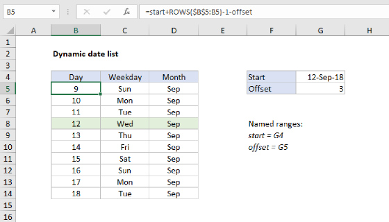
With the first day established in B6, the other formulas in the grid simply increment the previous date by one, beginning with the formula in C6:

=IF(B6<>"",B6,$H5)+1

This formula tests the cell immediately to the left for a value. If no value is found, it pulls a value from column H in the row above. Note $H5 is a mixed reference, to lock the column as the formula is copied throughout the grid. The same formula is used in all cells except B6.

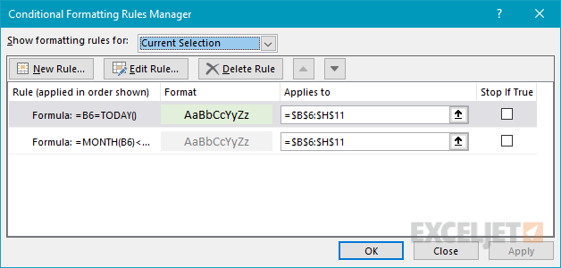
Conditional formatting rules

The calendar uses conditional formatting formulas change formatting to shade previous and future months, and to highlight the current day. Both rules are applied to the entire grid. For for previous and next months, the formula is:

=MONTH(B6)<>MONTH(start)

For current day, the formula is:

=B6=TODAY()

Conditional formatting rules for dynamic calendar

For more details, see: Conditional formatting with formulas (10 examples)

Calendar heading

The calendar title – month and year – are calculated with this formula in cell B4:

=start

Formatted with the custom number format "mmmm yyyy". To center the title above the calendar, the range B4:H4 has horizontal alignment set to "center across selection". This is a better option than merge cells, since it doesn't alter the grid structure in the worksheet.

Perpetual calendar with current date

To create a calendar that updates automatically based on the current date, you can use formula like this in K5:

=EOMONTH(TODAY(),-1)+1

This formula gets the current date with the TODAY function, then gets the first day of the current month using the EOMONTH function. Replace TODAY() with any given date to build a calendar in a different month. More details on how EOMONTH works here.