Highlight dates that are weekends

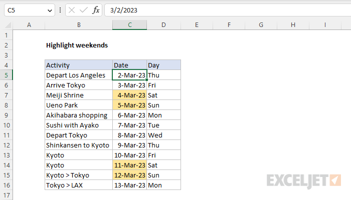
To highlight dates that land on weekends (i.e. Saturday or Sunday) with conditional formatting, you can use a simple formula based on the WEEKDAY function and the OR function. In the example shown, weekend dates are highlighted with the following formula:

=OR(WEEKDAY(C5)=7,WEEKDAY(C5)=1)

Once you save the rule, you'll see all dates that are a Saturday or a Sunday highlighted by your rule. If the dates in the data are changed, the highlighting will update instantly.

Explanation

In this example, the goal is to highlight dates that occur on weekends. In other words, we want to highlight dates that land on either Saturday or Sunday. This problem can be easily solved by applying conditional formatting with a formula based on the WEEKDAY function together with the OR function.

WEEKDAY function

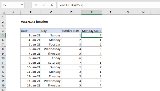
The WEEKDAY function takes a date and returns a number between 1-7 representing the day of week. By default, WEEKDAY returns 1 for Sunday and 7 for Saturday. For example, with the date January 16, 2023 in cell A1, WEEKDAY will return 2, since the day of week is Monday:

=WEEKDAY(A1) // returns 2

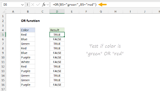
OR function

The OR function returns TRUE if any given arguments evaluate to TRUE, and returns FALSE only if all supplied arguments evaluate to FALSE. For example, if cell A1 contains the text "apple", then:

=OR(A1="pear",A1="apple") // returns TRUE
=OR(A1="pear",A1="orange") // returns FALSE

We can combine the WEEKDAY function with the OR function to test for weekends as explained below.

Test for weekends

To highlight weekends, we need a formula that will return TRUE if a date is either Saturday or Sunday. We can do that by combining the WEEKDAY function with the OR function like this:

=OR(WEEKDAY(C5)=7,WEEKDAY(C5)=1)

Inside the OR function, WEEKDAY returns a number between 1 and 7. If WEEKDAY returns either 7 or 1, the OR function will return TRUE. In all other cases, OR will return FALSE. This is what we need to trigger a conditional formatting rule.

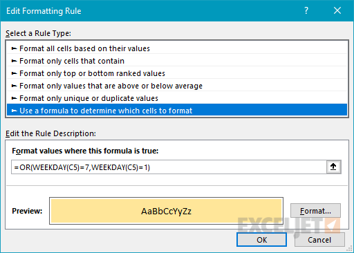
Define the rule

The next step is to define the conditional formatting rule itself. With the range C5:C16 selected, navigate to Home > Conditional Formatting > New rule. Then select "Use a formula to determine which cells to format". Next, enter the formula above in the formula area and set the desired format. At this point, the conditional formatting rule should look like this:

Conditional formatting rule to highlight weekends

Video: How to apply conditional formatting with a formula

Highlighting the entire row

The rule above will highlight dates in C5:C16 only. To highlight the entire row when a date is a weekend, start by selecting all data in the range B5:D16. Then use a modified formula that locks the date column:

=OR(WEEKDAY($C5)=7,WEEKDAY($C5)=1)

Note in this version of the formula, $C5 is a mixed reference with the column locked. We do this because we want to make sure that the test for weekend dates is always applied to the dates in column C.