Summary
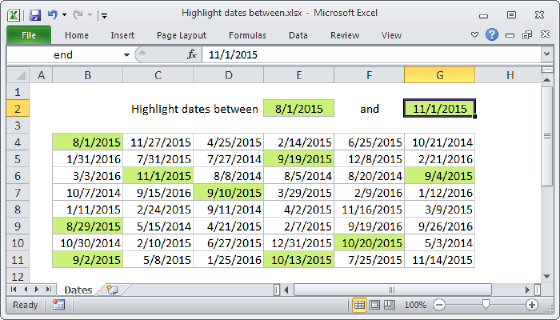
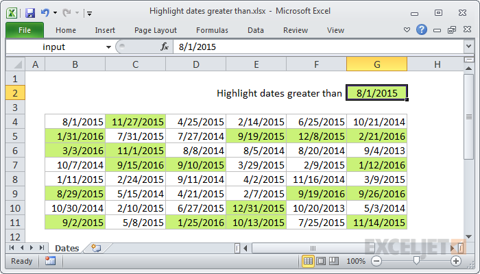
If you want to highlight dates greater than or less than a certain date with conditional formatting, you can use a simple formula that relies on the date function. For example, if you have dates in the cells B4:G11, and want to highlight cells that contain a date greater than August 1st, 2015, select the range and create a new CF rule that uses this formula:
=B4>DATE(2015,8,1)
Note: it's important that CF formulas be entered relative to the "active cell" in the selection, which is assumed to be B4 in this case.
Once you save the rule, you'll see the dates greater than 8/1/2015 are highlighted.
Generic formula
=A1>DATE(year,month,day)
Explanation
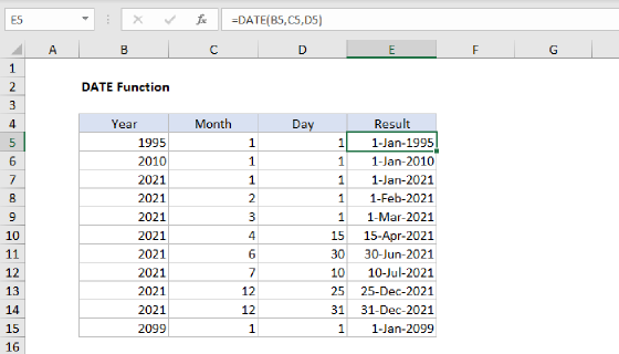
The DATE function creates a proper Excel date with given year, month, and day values. Then, it's simply a matter of comparing each date in the range with the date created with DATE. The reference B4 is fully relative, so will update as the rule is applied to each cell in the range, and any dates greater than 8/1/2015 will be highlighted.
Greater than or equal to, etc.
Of course, you can use all of the standard operators in this formula to adjust behavior as needed. For example, to highlight all dates greater than or equal to 8/1/2015, use:
=B4>=DATE(2015,8,1)
Use another cell for input
There is no need to hard-code the date into the rule. To make a more flexible, interactive rule, use another cell like a variable in the formula. For example, if you want to use cell C2 as an input cell, name cell C2 "input", enter a date, and use this formula:
=B4>input
Then change the date in cell C2 to anything you like and the conditional formatting rule will respond instantly.