Summary
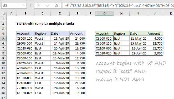
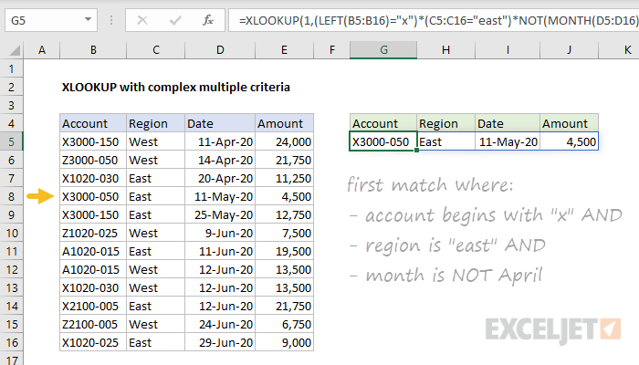
To lookup data based on multiple complex criteria, you can use the XLOOKUP function with multiple expressions based on Boolean logic. In the example shown, the formula in G5 is:
=XLOOKUP(1,(LEFT(B5:B16)="x")*(C5:C16="east")*NOT(MONTH(D5:D16)=4),B5:E16)
With XLOOKUP's default settings for match_mode (exact) and search_mode (first to last) the formula matches the first record where:
account begins with "x" AND region is "east", and month is NOT April.
The first match is the fourth record (row 8) in the example shown.
Explanation
Normally, the XLOOKUP function is configured to look for a value in a lookup array that exists on the worksheet. However, when the criteria used to match a value becomes more complex, you can use Boolean logic to create a lookup array on the fly composed only of 1s and 0s, then look for the value 1. This is the approach used in this example:
=XLOOKUP(1,boolean_array,result_array)
In this example, the required criteria is:
account begins with "x" AND region is "east", and month is NOT April.
For each of the three separate criteria above, we use a separate logical expression. The first expression uses the LEFT function to test if the Account begins with "x":
LEFT(B5:B16)="x" // account begins with "x"
Because we are checking 12 values, the result is an array with 12 TRUE FALSE values like this:
{TRUE;FALSE;TRUE;TRUE;TRUE;FALSE;FALSE;FALSE;TRUE;TRUE;FALSE;TRUE}
The second expression tests if Region is "east" using the equal to (=) operator:
C5:C16="east" // region is east
As before, we get another array with twelve TRUE FALSE values:
{FALSE;FALSE;TRUE;TRUE;TRUE;FALSE;TRUE;FALSE;FALSE;TRUE;FALSE;TRUE}
The third expression needs to exclude the month of April. The easiest way to do this is to test for the month of April directly with the MONTH function:
MONTH(D5:D16)=4 // month is April
Then use the NOT function to reverse the result:
NOT(MONTH(D5:D16)=4) // month is not April
which creates an array correctly describing "not April":
{FALSE;FALSE;FALSE;TRUE;TRUE;TRUE;TRUE;TRUE;TRUE;TRUE;TRUE;TRUE}
Next, all three arrays are multiplied together, and the math operation coerces the TRUE and FALSE values to 1s and 0s:
{1;0;1;1;1;0;0;0;1;1;0;1}*
{0;0;1;1;1;0;1;0;0;1;0;1}*
{0;0;0;1;1;1;1;1;1;1;1;1}
In Boolean arithmetic, multiplication works like the logical function AND, so the final result is a single array like this:
{0;0;0;1;1;0;0;0;0;1;0;1}
The formula can now be rewritten like this:
=XLOOKUP(1,{0;0;0;1;1;0;0;0;0;1;0;1},B5:E16)
With 1 as a lookup value, and default settings for match_mode (exact) and search_mode (first to last), XLOOKUP matches the first 1 (fourth position) and returns the corresponding row in the result array, which is B8:E8.
Last match
By setting the optional search mode argument to -1, you can locate the "last match" with the same criteria like this:
=XLOOKUP(1,(LEFT(B5:B16)="x")*(C5:C16="east")*NOT(MONTH(D5:D16)=4),B5:E16,,,-1)
Dynamic Array Formulas are available in Office 365 only.