Summary
To configure XLOOKUP with Boolean OR logic, use a lookup value of 1 with a logical expression based on addition. In the example shown, the formula in G5 is:
=XLOOKUP(1,(data[Color]="red")+(data[Color]="pink"),data)
where data is the name of the Excel Table in the range B5:E14.
Note: see below for an equivalent formula based on INDEX and MATCH.
Generic formula
=XLOOKUP(1,boolean_expression,data)
Explanation
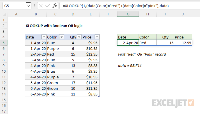
In this example, the goal is to use XLOOKUP to find the first "red" or "pink" record in the data as shown. All data is in an Excel Table named data in the range B5:E14. This means the formulas below use structured references. As a result, the formulas will automatically include new data added to the table.
XLOOKUP function
In the worksheet shown, the formula in cell G5 is:
=XLOOKUP(1,(data[Color]="red")+(data[Color]="pink"),data)
The lookup_value is provided as 1, for reasons that become clear below. For the lookup_array, we use an expression based on Boolean logic:
(data[Color]="red")+(data[Color]="pink")
In the world of Boolean algebra, AND logic corresponds to multiplication (*), and OR logic corresponds to addition (+). Because we want OR logic, we use addition in this case. Notice Excel is not case-sensitive, so we don't need to capitalize the colors.
After the expression is evaluated, we have two arrays of TRUE and FALSE values like this:
{FALSE;FALSE;TRUE;FALSE;FALSE;FALSE;FALSE;FALSE;FALSE;FALSE}+
{FALSE;FALSE;FALSE;FALSE;TRUE;FALSE;FALSE;FALSE;FALSE;TRUE}
Notice, in the first array, TRUE values correspond to "red". In the second array, TRUE values correspond to "pink".
The math operation of adding these arrays together converts the TRUE and FALSE values to 1s and 0s, and results in a new array composed only of 1s and 0s:
{0;0;1;0;1;0;0;0;0;1}
Notice the 1s in this array correspond to rows where the color is either "red" or "pink". We can now rewrite the formula like this:
=XLOOKUP(1,{0;0;1;0;1;0;0;0;0;1},data)
The first 1 in the lookup array corresponds to row three of the data, where the color is "red". Since XLOOKUP will by default return the first match, and since the entire table data is supplied as the return array, XLOOKUP returns the third row as a final result.
Not mutually exclusive
In the example above, we are testing for two possible values in a single column of data. This means the values are mutually exclusive — both tests can't return TRUE at the same time. If you are testing multiple columns/fields for values, or if the tests are otherwise not mutually exclusive, the formula logic needs to be adjusted to handle the possibility that more than one logical test will return TRUE. In that case, when the result arrays are added together, the final array will contain a number larger than 1 and the lookup value of 1 will not be found. To guard against this problem, you can adjust the formula as follows:
=XLOOKUP(1,--((test1)+(test2)>0),array)
In this version, we add result arrays together and check to see if the results are greater than 0. This creates a new array containing only TRUE and FALSE values. The double negative (--) is used to convert the TRUE and FALSE values to 1s and 0s so the lookup value of 1 will continue to work.
For example, in the worksheet shown, to test for the first record with a color of "green" OR a quantity greater than 15, use a formula like this:
=XLOOKUP(1,--((data[Color]="green")+(data[Qty]>15)>0),data)
You can of course adjust the logic as needed to target the desired data.
Video: Boolean algebra in Excel.
INDEX and MATCH
In older versions of Excel that do not include the XLOOKUP function, you can perform the same lookup with an INDEX and MATCH formula:
=INDEX(data,MATCH(1,(data[Color]="red")+(data[Color]="pink"),0),0)
In this formula, the MATCH function uses the same logic explained above to locate the correct row number, which is returned to INDEX as the row_num argument. The column_num argument is hardcoded as 0 to tell the INDEX function to return the entire row.
Because this formula returns 4 values in one row, it must be entered as a multi-cell array formula in Legacy Excel. In Excel 365 and Excel 2022, the formula "just works" and all four values spill into multiple cells. For more on this behavior, see: Dynamic Array Formulas in Excel.
FILTER function
If you want to display all "red" or "pink" records, you can use the FILTER function with exactly the same logic like this:
=FILTER(data,(data[Color]="red")+(data[Color]="pink"))
Boolean logic works well in all the new Dynamic Array functions and is nicely portable — you can copy the lookup_array from XLOOKUP into FILTER as the include argument, and it just works.