Look up and return to single cell

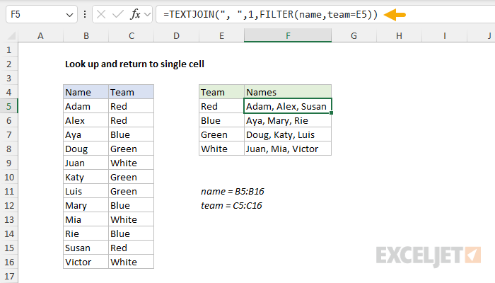
To look up and return all matches to a single cell, you can use a formula based on the FILTER function and the TEXTJOIN function. In the worksheet shown, the formula in cell F5, copied down, looks like this:

=TEXTJOIN(", ",1,FILTER(name,team=E5))

As the formula is copied down, it returns the names for each team in column E, separated by commas. Because the result is a single text string, it fits neatly into one cell without spilling. For convenience only, the worksheet contains two named ranges: name (B5:B16) and team (C5:C16).

Explanation

In this example, the goal is to look up and retrieve all names for a given team and return them in a single cell as a comma‑separated list. At the core, this is a lookup problem, but the twist is that we want to return multiple matches for each team, not just one. That means traditional lookup functions like VLOOKUP, XLOOKUP, etc., won't work because they only return the first match. Although this example deals with team members, it is applicable to many other real-world problems, including:

Project staffing – list everyone assigned to the same project code.
Class schedules – show all students in a given class period.
Class list - show all classes for a given student.
Sales analysis – list products in the same category.

What makes the task unique is that we want to locate multiple matches (i.e., all members of a given team), but we the result to be delivered to a single cell formatted as a clean, readable list (i.e., “Doug, Katy, Luis”) instead of a block names in different cells. In this article, we’ll explore two ways to solve the problem:

FILTER + TEXTJOIN – simple and flexible
GROUPBY + LAMBDA – an all‑in‑one summary table

We'll also look at replacing TEXTJOIN with the ARRAYTOTEXT function to create even simpler formulas.

Note: For convenience only, the worksheet contains two named ranges: name (B5:B16) and team (C5:C16). Named ranges make the formulas below easier to read and write, but they are not required.

Option 1: FILTER and TEXTJOIN

A straightforward solution to this problem is to use a formula based on the FILTER function combined with the TEXTJOIN function. This is the approach seen in the worksheet above, where the formula in F5 is:

=TEXTJOIN(", ",1,FILTER(name,team=E5))

At a high level, this formula uses FILTER to look up the names for a given team, and TEXTJOIN to join the names together with commas. Working from the inside out, FILTER is configured like this:

FILTER(name,team=E5)

In this configuration, name (B5:B16) is the array argument, which represents the values to return. The expression team=E5 is the include argument, which returns a Boolean array where each value is TRUE if the corresponding team matches the value in E5. FILTER uses this array to return only the names associated with the selected team. Since the team in E5 is “Red”, FILTER returns an array in the form {"Adam";"Alex";"Susan"} as a result. This array is returned directly to the TEXTJOIN function as the text1 argument. Simplifying, the formula becomes:

=TEXTJOIN(", ",1,{"Adam";"Alex";"Susan"})

Here, the delimiter is set to a comma and a space to separate values, and the ignore_empty argument is set to 1 (or TRUE) to ignore any empty values. Finally, TEXTJOIN concatenates the values using “, ” as a delimiter:

"Adam, Alex, Susan"

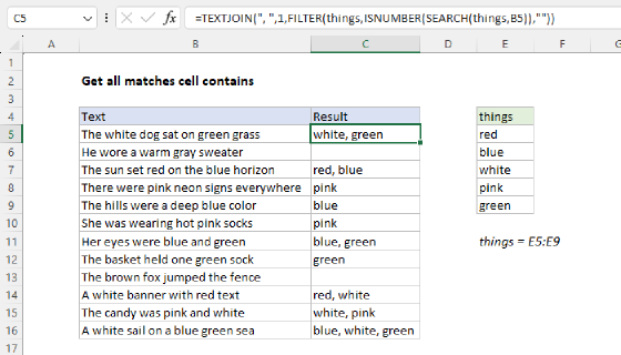
Because the result is a single text string, it fits neatly into one cell without spilling. As the formula is copied down, it returns names for each of the remaining teams. A key advantage of this approach is the flexibility provided by FILTER. Although we are using FILTER to test for an exact match on team name, this logic could be easily adjusted to suit other situations. For example, you could adjust FILTER to test for cells that contain "red" with a generic formula like this:

=FILTER(range,ISNUMBER(SEARCH("red",range)))

For details on the formula above, see: FILTER text contains. See our main FILTER page for more examples of how filter logic can be extended.

Listing team names

The formula above assumes that teams are already listed in column E. You can either enter the team names manually or retrieve them with another formula. To get a list of unique teams with a formula, you can use the UNIQUE function like this in cell E5:

=UNIQUE(C5:C16)

UNIQUE will return the team names as shown, and then you can use the formula based on FILTER and TEXTJOIN.

Option 2: GROUPBY and LAMBDA

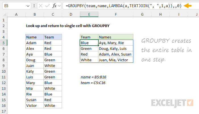
Another option for solving this problem is to use the new GROUPBY function, which essentially builds a lightweight pivot table with a formula. With GROUPBY, you can build the entire summary table with one formula like this in cell E5:

=GROUPBY(team,name,LAMBDA(a,TEXTJOIN(", ",1,a)),,0)

Using GROUPBY to create the entire summary in one step

This is a great formula to demonstrate the flexibility and power of GROUPBY. The basic configuration looks like this:

row_fields – team (C5:C16)
values – name (B5:B16)
function – custom LAMBDA, explained below
field_headers – not provided
total_depth – 0 (no totals)

At a high level, we are grouping the names by teams. For the calculation, we are using a custom LAMBDA that joins names together, separated by commas, using the TEXTJOIN function. The total depth is set to zero because we don't want totals. Let’s look at the custom LAMBDA in more detail:

LAMBDA(a,TEXTJOIN(", ",1,a))

The first argument, a, stands for the array of names in each group. The second part is the TEXTJOIN function, configured to join the values in a using a comma and space. We have also set the ignore_empty argument to 1 (TRUE) to ignore any empty values that might creep into the array. This could happen if a team appeared in column B, but the corresponding cell in column C was empty.

At a high level, the GROUPBY function gathers names by team and feeds the resulting arrays into the LAMBDA. The LAMBDA then joins the values separated by commas using TEXTJOIN. The result is a two-column table that lists every unique team alongside the names associated with that team. A nice advantage of this approach is that there is no separate step to get a list of unique teams. The GROUPBY function handles that automatically. This makes GROUPBY ideal for dashboards or pivot-table-style summaries that need to accommodate changing data.

The idea of a "custom LAMBDA" sounds complicated. However, as you can see above, custom LAMBDAs can be quite simple. You will see them pop up frequently in other functions like GROUPBY, PIVOTBY, BYCOL, and BYROW that need to loop over data and perform a specific operation that requires some configuration. They are simply a generic container to deliver a custom calculation.

ARRAYTOTEXT option

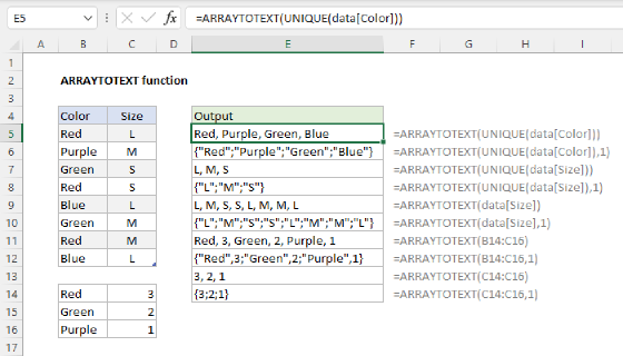
An interesting way to make the formulas above simpler is to use the ARRAYTOTEXT function instead of the TEXTJOIN function. ARRAYTOTEXT is a utility function that converts an array or range into a text string. You can use ARRAYTOTEXT as a shortcut when the goal is to return comma-separated text. Below are the formulas above modified to use the ARRAYTOTEXT function:

=ARRAYTOTEXT(FILTER(name,team=E5))
=GROUPBY(team,name,ARRAYTOTEXT,,0)

As you can see, ARRAYTOTEXT is a drop-in replacement for the TEXTJOIN function, and it doesn't even require configuration, which makes both formulas notably shorter. This works because ARRAYTOTEXT will automatically output comma-separated text by default. However, one thing to remember with the ARRAYTOTEXT function is that its delimiters are based on regional settings, which vary by user. For example, if regional settings are for French/France, you will see semicolons (;) instead of commas. The other potential issue is that ARRAYTOTEXT has no way to suppress empty values, which will appear in the output as a repeated delimiter. If you need to define delimiters precisely or ignore empty values, TEXTJOIN is a better option.

Summary

In this article, we looked at two ways to perform a lookup in Excel and return all matches to a single cell:

FILTER + TEXTJOIN is a flexible everyday solution. It’s short, transparent, and easy to adapt. It's a bit more work to set up because we need to get a list of unique teams first in column E, but it's easier to understand.
GROUPBY + LAMBDA goes further, producing a complete one-formula summary table. The main advantage is that you get the entire summary in one formula. The trade-off is that the formula is a bit harder to read and understand.

For simplicity, the examples above use simple static ranges in all formulas. However, if you have a lot of data or if the data changes frequently, you may want to use an Excel Table as the source. Another is to use a dynamic range created with the TRIMRANGE function. In both cases, the ranges will be dynamic. This means the table will instantly update as rows are added or removed.