TRIMRANGE Function

The TRIMRANGE function removes empty rows and columns from a range of data. Given a range or array, it will exclude empty rows and/or columns and return a "trimmed" range that contains only data. The beauty of TRIMRANGE is that it will track the data in a worksheet as it changes. When data is added or removed, the range will automatically adjust, with no need to adjust cell references manually. This means you can feed the result from TRIMRANGE into other formulas, and they will always use the latest data to calculate results. For this reason, TRIMRANGE is a good option for creating a dynamic range, or a dynamic named range, with a formula. See below for details with examples.

TRIMRANGE and Trim References (also called "Trim Refs") are two different ways to accomplish the same thing. This article is focused on TRIMRANGE, but includes a section on Trim Refs below.

Table of Contents

• Basic syntax
• Alternative Trim refs syntax
• How TRIMRANGE works
• What is a dynamic range?
• Example - Trimming a large range
• Example - Creating a dynamic range
• Example - Creating a dynamic named range
• Example - Creating a dropdown menu
• Example - Anchoring other formulas
• Key benefits of TRIMRANGE
• When to use TRIMRANGE
• Tips for using TRIMRANGE
• TRIMRANGE limitations
• Notes on TRIMRANGE

Basic syntax

The syntax for TRIMRANGE is simple; just give it a range, and it will automatically remove empty rows and columns:

=TRIMRANGE(range) // remove empty rows and columns

There are two optional arguments, trim_rows, and trim_columns, that let you fine-tune this behavior:

=TRIMRANGE(range,1,1) // remove leading rows and columns
=TRIMRANGE(range,2,2) // remove trailing rows and columns
=TRIMRANGE(range,1,2) // remove leading rows and trailing columns

In each case, TRIMRANGE will examine the data in the range and discard empty rows and/or columns outside the data. The result is a "trimmed range" that includes only the data in the original range. Like other Excel formulas, TRIMRANGE is dynamic, so the result will automatically update to match changes in the worksheet.

Alternative Trim Refs syntax

When the Excel team added TRIMRANGE to Excel, they also added "Trim references" (also called "Trim refs") to Excel's list of range operators. Essentially, trim refs use a dot (.) together with the colon (:) in a range to add trim behaviors. Here are some examples:

=A:F // normal range, not trimmed
=A:.F // trim trailing rows and columns
=A.:F // trim leading rows and columns
=A.:.F // trim leading and trailing rows and columns

Note: Trim refs are an alternative to TRIMRANGE — don't use TRIMRANGE and trim refs together; use one or the other. Personally, I prefer the TRIMRANGE function because it makes the action clear and explicit. The dot syntax is tricky to read and might not be noticed or understood by many users.

How TRIMRANGE works

It's important to understand how TRIMRANGE works. Starting from the outer boundary of the range, TRIMRANGE scans inward. When it finds a non-blank value, it uses it as a reference point and discards the empty rows or columns between the reference point and the outer boundary. Depending on how TRIMRANGE is configured, this process is repeated for the incoming array's top, bottom, right, and left edges. The result is a rectangular range that includes all data contained by the original range, with the empty rows and columns around the data "trimmed off". You can see the basic concept in the worksheet below, we are using TRIMRANGE like this:

=TRIMRANGE(A:J)

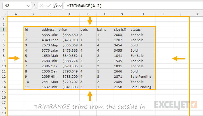
Starting with the full column reference A:F, TRIMRANGE trims from the outside in. It removes empty leading and trailing rows, and empty leading and trailing columns. The final result is data in the range B3:H14. 

Important: TRIMRANGE does not remove any empty rows or columns from the interior of a set of data, it only removes unused rows and columns outside the rectangle that contains the data.

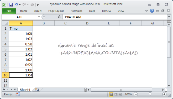
What is a dynamic range?

To understand why TRIMRANGE can be useful, you should understand the concept of a dynamic range. A dynamic range in Excel automatically expands and contracts to track the data it contains. This kind of range is useful for things like reports, pivot tables, and charts that need to process data that is always changing. There are a variety of ways to create a dynamic range in Excel, including:

• Excel Tables - The easiest way to create a dynamic range in Excel. You can create an Excel Table with the shortcut Control + T, then give the table a name. Excel Tables are designed to expand as needed to contain all data automatically. They work well, but they do have a few limitations. They can't contain dynamic array formulas, and headers in a table must be unique. For a full rundown, see our guide to Excel Tables.
• Spill range - Modern dynamic array formulas can create a spill range, which can be used as a simple dynamic range. For example, if you use the UNIQUE function in cell A1, you can refer to the values returned by UNIQUE with the syntax =A1#. This reference will track the data returned by UNIQUE as it changes. One key limitation of spill ranges is that they only contain values generated by a formula, they don't contain data entered manually on a workbook.
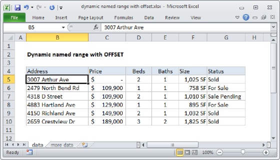
• Regular Formula - the classic way to create a dynamic range is to use the name manager to create a name that is defined by a regular formula. Traditionally, this formula uses a function like OFFSET (example) or INDEX (example) to compute a range by counting values in a worksheet and using those counts to construct a range from a given starting point. Formulas like this pre-date Excel Tables and can work pretty well. However, they are complicated and non-intuitive to most users. The OFFSET version can also cause performance problems because OFFSET is a volatile function that automatically recalculates with every workbook change.
• TRIMRANGE - the new TRIMRANGE function provides a new way to create a dynamic range with a simple formula. The beauty of TRIMRANGE is that you can give it a simple reference like A:C, and it will automatically return only the used portion of the range. Even better, there is no restriction on the data contained by the range. You can use any combination of formulas and manually entered data, and TRIMRANGE will happily return the portion of the range that contains that data.

Example - Trimming a large range

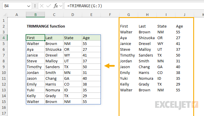
The main function of TRIMRANGE, as the name suggests, is to "trim" a range, which means to remove empty rows and columns outside a block of data. You can see an example of this in the worksheet below, where we have data in columns G through J, and we are using TRIMRANGE to trim the range down to only the rows that contain data. The formula in B4 looks like this:

=TRIMRANGE(G:J)

This is an example of using full-column references to simplify range management. The beauty of this approach is simplicity. Instead of working out the address of the last row that contains data, we just provide columns. However, we must be careful because Excel worksheets are very large — each worksheet contains over 1 million rows. When we use a range like G:J, we are referencing over 4 million cells since 1,048,576 rows * 4 columns = 4,194,304 cells. References like this can cause serious performance problems in certain worksheets because they can cause Excel to do a lot of extra work. Essentially, TRIMRANGE allows us to have our cake and eat it too. We can use simple references and let TRIMRANGE figure out which cells contain data.

In the worksheet, TRIMRANGE "trims" the range G:J by removing the empty rows above and below the data and returns the result as an array that lands in cell B4 and spills into the range B4:E15. Of course, this is a contrived example, so you can see how TRIMRANGE works on a small data set. More commonly, you will pipe the result of TRIMRANGE into another function. For example, to count rows of data in the range G:J, we can wrap TRIMRANGE in the ROWS function like this:

=ROWS(TRIMRANGE(G:J)) // returns 12

The result is 12, since there are 11 rows of data plus the header row. If we want to count rows of data only, we can use the DROP function to "drop" the first row like this:

=ROWS(DROP(TRIMRANGE(G:J),1)) // returns 11

The result from TRIMRANGE is dynamic. As data is added or removed from G:J, TRIMRANGE will continue to return the latest data in the used portion of the original range.

By default, TRIMRANGE trims empty rows and columns from a range. If we provided a larger range in the formulas above, like G:M, the result would be the same. TRIMRANGE would remove the unused rows above and below the data and also remove the three empty columns to the right.

Example - Creating a dynamic range

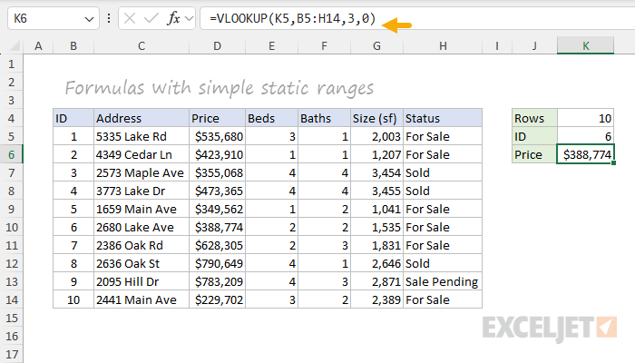
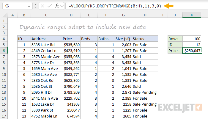
In this example, the goal is to create a simple dynamic range to track property listings, as seen in the worksheet below. The table that holds the property listings appears in the range B4:H14. The first row is a header row, so the actual data range is B5:H14. The formula in cell K4 uses the ROWS function to count the number of rows in the data:

=ROWS(B5:H14) // returns 10

Cell K5 is meant to hold a unique ID for a property, and cell K6 contains a VLOOKUP formula that uses the ID in K5 to look up the price for a given property:

=VLOOKUP(K5,B5:H14,3,0) // returns $388,774

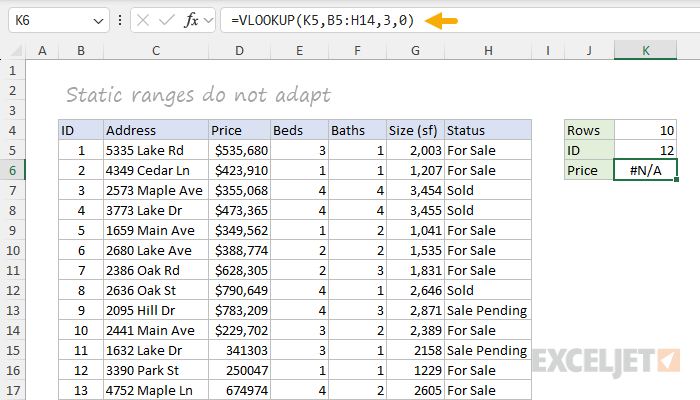
The result is $388,774, the correct price for property 6. Note that these ranges are not dynamic. If we paste in an additional 90 rows of data, and change the ID to 12, the row count in cell K4 doesn't change, and VLOOKUP returns #N/A since ID 12 does not exist in the range B5:B14, as you can see below:

The problem is that our original formula ranges are static and do not adjust to the new data. One way to make these ranges dynamic is to use the TRIMRANGE function with a range like B:H. Then, we replace the hardcoded range inside the ROWS function with TRIMRANGE like this:

=ROWS(TRIMRANGE(B:H)) // returns 101

Now, TRIMRANGE removes the empty rows from this (huge) range and returns a trimmed array to ROWS, which returns 101. This doesn't quite work in this case because we are including the header row together with the data. We can solve that problem by adding the DROP function to drop the first row. Now, ROWS returns 100, which is correct:

=ROWS(DROP(TRIMRANGE(B:H),1)) // returns 100

To adapt the VLOOKUP formula, we can use exactly the same approach, replacing the static range B5:B14 with the DROP + TRIMRANGE combo above:

=VLOOKUP(K5,DROP(TRIMRANGE(B:H),1),3,0)

You can see the result of these new formulas in the worksheet below:

What have we accomplished here? Well, the key improvement is that our formulas will now track the data correctly when rows are added or removed because they use dynamic ranges. In addition, using TRIMRANGE like this ensures we aren't processing more cells than needed, avoiding potential performance problems in large, complicated workbooks. It's a bit annoying to clutter up our simple reference to B:H with TRIMRANGE and DROP, but it works nicely. The next logical step is to create a dynamic named range.

Example - Creating a dynamic named range

In the previous example, we looked at how to adapt formulas using a static range to formulas using a dynamic range using the TRIMRANGE function with some help from the DROP function. This worked well, but one issue is that we need to keep typing out the code that created the dynamic range:

=DROP(TRIMRANGE(B:H),1)) // dynamic range

It would be nice if we could avoid this duplication. One way to do that is to create a named range. A named range is simply a human-readable name assigned to a range. Names ranges are cool, because they give you a way to create names for different parts of a worksheet that you can refer to in formulas. While many named ranges point to a static range like A1:A100, a formula can also be used to define the range. Because formulas respond to changes in a worksheet, we call this a "dynamic named range". To illustrate how this works, let's build on the previous example and create a dynamic named range called "data".

The first step is to define a name. Open the Name Manager with the keyboard shortcut Control + F3 (or navigate to Formulas > Name Manager in the ribbon), then click "New". Next, type the name "data", then enter the formula below:

=DROP(TRIMRANGE(Sheet3!$B:$H),1)

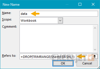
Note that we must use the absolute reference $B:$H when created a named range. This is because we need to the reference to work the same from any cell in the workbook. Excel will automatically add the sheet reference and cerate an absolute reference absolute if you point and click on the worksheet to select the range.

Now that we have created a named range, we can adapt our two existing formulas to use the name "data":

=ROWS(data)
=VLOOKUP(K5,data,3,0)

You can see these formulas in action in the worksheet below. Both formulas are now using the named range "data":

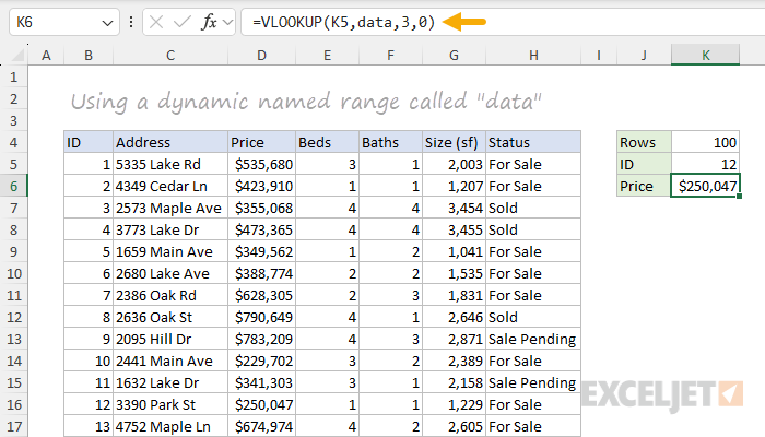
There are two key benefits to this approach. First, we have reduced redundant code in our formulas. Instead of two formulas that use TRIMRANGE + DROP in the same way, we have just one formula that defines the dynamic range in one location. Second, we have created a simple human-readable name, "data", that can be used by other formulas that need to refer to the same data. As before, the range is fully dynamic and will adapt as the worksheet is changed.

Example - Creating a dropdown menu

One interesting use of TRIMRANGE is to create a dropdown menu of preselected values using Data Validation with a formula to provide the list. You can see an example of this in the worksheet below, where both Products and Colors are set up as dropdown menus.

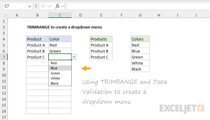
In this worksheet, we use Data Validation set to allow a List, and we use a TRIMRANGE formula to define the values in Source. The formula that creates values for the "products" list looks like this:

=DROP(TRIMRANGE($E:$E),1)

The formula that creates values for the "colors" list looks like this:

=DROP(TRIMRANGE($G:$G),1)

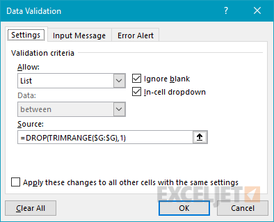
Both formulas use the DROP function to remove the header for each list that appears in row 4. Because we are using TRIMRANGE, these formulas are dynamic and will instantly update when products or colors change. 

Note we are not using TRIMRANGE to create a dynamic named range in this case but we could. The exact same formulas above can be used to create the names "products" and "colors" and then these names can be used directly the Data Validation rule instead of the formulas. In addition to being a bit more friendly, creating named ranges would make sense if there was a need to use the same lists elsewhere in the workbook. For more details on Data Validation, see this page.

Example - Anchoring other formulas

Another use of TRIMRANGE is to "anchor" other formulas. What does this mean, exactly? In the current version of Excel, formulas that return multiple values will spill onto the worksheet, creating a spill range. For example, in the worksheet below, we can use the LEN function to calculate the length of each text string in column B with one formula in cell D5 like this:

=LEN(B5:B15)

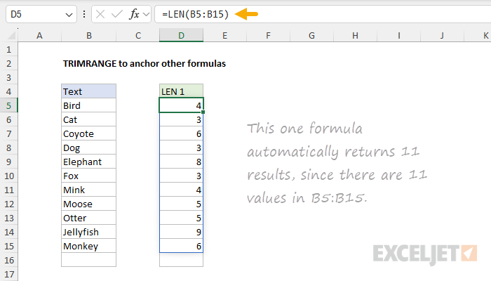
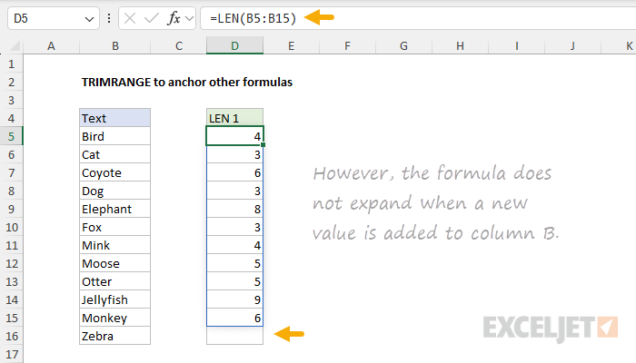
Because there are 11 values in the range B5:B16, LEN will return 11 results in an array that spills onto the worksheet. This is convenient because we get all 1 results with a single formula. However, if we add another value to column B, the formula above will not expand because the range B5:B15 will not change:

This takes the fun out of using a formula like this. So, how can we get a simple formula like this to expand when new data is added to column B? With TRIMRANGE, naturally 🙂. In the worksheet below, we have the original formula in cell D5. In cell E5, we have a new formula that incorporates TRIMRANGE like this:

=LEN(DROP(TRIMRANGE(B:B),3))

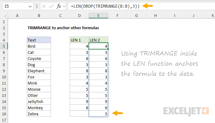
In this formula, TRIMRANGE first removes the empty rows above and below the data in column B, so that we are only working with the used portion of the range. Next, TRIMRANGE returns the trimmed range to the DROP function, which is configured to remove the first 3 rows. The result is a truncated array that contains the 12 text strings in B5:B16, which DROP returns to LEN. Finally, the LEN function counts the characters in each value and returns 12 results, which spill into the range E5:E16. The difference is that the LEN formula is "anchored" to the data in column B because we are using TRIMRANGE. As values are added and removed to column B, the LEN formula will automatically expand or contract as needed.

Note our use of DROP in this case is different from the other formulas explained above because we need to remove three rows and not just one. This may seem a bit confusing since there are actually 4 rows above cell B5 that we want to discard. However, remember that TRIMRANGE trims the range first, before DROP gets involved. That means the first row is already gone by the time the range gets to DROP, so we only need to remove three rows. There are different ways to handle this kind of problem. We could for example, use TRIMRANGE by itself with a smaller range like B5:B1000 that starts at the first value. However, in a "busy" worksheet, you will start to see this reference change if rows are inserted or deleted. What makes a reference like B:B nice is that it is stable and unaffected by common editing tasks.

Key benefits of TRIMRANGE

TRIMRANGE is a technical function designed for more advanced users. Potential benefits include:

• The ability to use very simple references like A:F without performance problems.
• A simple way to create a dynamic range in Excel.
• A way to speed up slow workbooks that use large, inefficient references.
• A way to provide trimmed ranges to other functions.
• A way to clean up messy ranges before handing off to other tools.

When to use TRIMRANGE

Here are some situations where you may want to use TRIMRANGE:

• You want to trim off extra (unused) rows or columns from a range.
• You want to use a reference like =A:Z because you don't know how many rows or columns to expect.
• You want a simple dynamic range, but you don't want to use an Excel Table.
• You want to simple named range that dynamically expands to include new data.
• You want to fix a performance problem caused by large references that trigger too much calculation.

Tips for using TRIMRANGE

• When you use full-column references like A:F with trim range, make sure that there is no other data below the data you are targeting. If there is, TRIMRANGE will include this extra data in your range. For example, if you have 200 rows of data starting at row 1, and there's a cell in A9000 that contains a single character like "x", TRIMRANGE will see this content and expand the range to include 9000 rows. Even a cell with a single (invisible) space can cause this problem.
• If you are working with a messy spreadsheet that has been used by many people, a good way to clean things up fast is to simply delete all rows below the data before you use TRIMRANGE. This will clear out any wayward junk that might be lurking in the cells below. First, make sure there is nothing important below the data, then select an entire row below the data, extend the selection to the bottom of the worksheet, and delete the rows. You can do the same thing with columns to the right. Select an entire column to the right of the data, extend the selection to the right edge of the worksheet, and delete all columns. When you delete rows and columns like this, Excel simply replaces them with fresh copies, so your worksheet stays the same size.

TRIMRANGE limitations

• TRIMRANGE does not currently work with 3D references like =Sheet1:Sheet3!A:A. 
• TRIMRANGE cannot be used directly to create a dynamic Pivot Table. However, you can use TRIMRANGE to create a named range like "data" (explained above) and then use the named range as the Pivot Table source.

Notes on TRIMRANGE

• If the target range contains no data, TRIMRANGE returns a #REF! error.
• TRIMRANGE trims empty rows and columns dynamically based on the data in the range.
• Useful for creating dynamic ranges without Excel Tables.
• Can be used with other functions to handle data dynamically and efficiently.
• Does not work with 3D references.
• Offers a simple solution for managing large data sets without performance issues.