Purpose
Return value
Syntax
=TOROW(array,ignore,scan_by_column)- array - The array to transform.
- ignore - Control to ignore blanks and errors.
- scan_by_column - Scan array by column. TRUE = by column, FALSE = by row (default).
Using the TOROW function
The TOROW function transforms an array or range into a single row. TOROW can scan values by row, left to right (default) or by column, top to bottom.
The TOROW function takes three arguments: array, ignore, and scan_by_column. Array is the only required argument and represents the array or range to be transformed. The ignore argument controls what values TOROW will optionally ignore. The options for ignore are as follows:
| Value | Purpose |
|---|---|
| 0 (default) | Keep all values |
| 1 | Ignore blanks |
| 2 | Ignore errors |
| 3 | Ignore blanks and errors |
The scan_by_column argument is a boolean value that controls how TOROW reads values from the source array. By default, scan_by_column is FALSE and TOROW will read values "by row" from left to right. At the end of each row, TOROW will move down and read values from the next row in the same order. To read values instead by column, set scan_by_column to TRUE or 1. In this mode, TOROW will read values from top to bottom in the first column, then move one column to the right, and read the next column from top to bottom.
Use the TOROW function to transform an array into a single row and the TOCOL function to transform an array into a single row. The TRANSPOSE function will transpose an array from horizontal to vertical and vice versa, but it won't restructure the array.
Basic usage
By default, the TOROW function transforms a two-dimensional array into a single row, one row at a time. In the example below, the formula in F4 is:
=TOROW(B4:D5)

TOROW converts the 2 x 3 array in B4:D5 into the 1 x 6 array in F4:K4.
Note: in Excel, arrays map directly to ranges. Technically, the array is converted and the result lands in cell F4, where it spills into the range F4:K4.
Ignore blanks and errors
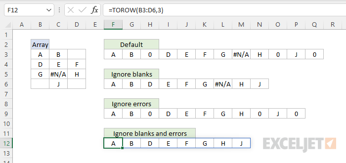
The ignore argument in TOROW can be set to ignore blanks and/or errors like this:
=TOROW(array,1) // ignore blanks
=TOROW(array,2) // ignore errors
=TOROW(array,3) // ignore blanks and errors
The screen below shows how these options work with the range B3:D6.

Scan by column
By default, TOROW will read values "by row" from left to right. To read values instead by column, set scan_by_column to TRUE or 1. The worksheet below shows the default "by row" behavior in F4. In cell F7, scan_by_column is set to TRUE:
=TOROW(B4:D5,,TRUE)

Notice the resulting array is the same size, but the values appear in a different order.


