=WRAPROWS(vector, wrap_count, [pad_with])- vector - The array or range to wrap.
- wrap_count - Max values in each row.
- pad_with - [optional] Value to use for unfilled places.
Using the WRAPROWS function
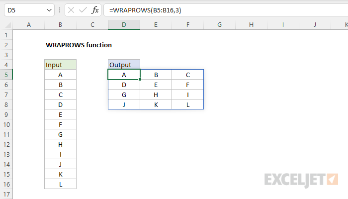
The WRAPROWS function converts a one-dimensional array into a two-dimensional array by wrapping values into separate rows. The length of each row is provided as the wrap_count argument: when the count is reached, WRAPROWS starts a new row.
The WRAPROWS function takes three arguments: vector, wrap_count, and pad_with. Vector and wrap_count are both required. Vector must be a one-dimensional array or range. Wrap_count is a number that represents the length of each row. The final argument, pad_with, is an optional value to use if there are unfilled places in the last row. If no value is supplied, WRAPROWS will return an #N/A error after all values in vector have been used, and there are still unfilled places in the resulting array. You can override this behavior by providing a custom value for the pad_with argument.
Basic usage
WRAPROWS outputs values "by row", working left to right, top to bottom. When wrap_count has been reached, WRAPROWS starts a new row. In the worksheet below, the goal is to wrap the range C2:J2 into 2 rows that each contain 4 values. The formula in B5 is:
=WRAPROWS(C2:J2,4)
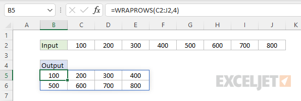
Notice WRAPROWS outputs values "by row", moving left to right, and each row contains 4 values.
Wrap count
Wrap_count represents the maximum number of values in each row. Once the count has been reached, WRAPROWS starts a new row. In the screen below, you can see how this works. The formula in D3 uses a wrap_count of 4:
=WRAPROWS(B3:B14,4)
The formula in D9 uses a wrap_count of 3:
=WRAPROWS(B3:B14,3)
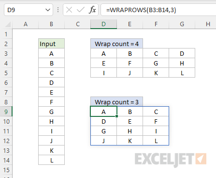
Notice values are output from left to right, and top to bottom.
Padding
If no value is supplied for pad_with, WRAPROWS will return an #N/A error after all values in the source array have been accounted for. You will see these errors appear in the last row when the size of the source array is not evenly divisible by the wrap_count. You can override this behavior by providing a custom value for the pad_with argument. The formula in D3 shows default behavior. No value for pad_with has been provided:
=WRAPROWS(B3:B12,4)
The input range contains only 10 cells, which is not evenly divisible by 4. As a result, the last 2 cells return #N/A. To override this behavior, provide a value for pad_with. The formula in D10 supplies "x" for pad_with:
=WRAPROWS(B3:B12,4,"x")
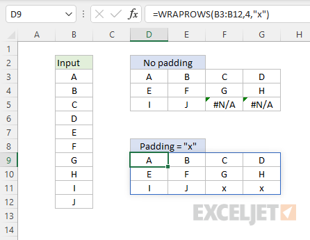
Notice the #N/A errors have been replaced by "x" in the resulting array.
Notes
- WRAPROWS will return a #VALUE! error if vector is not a one-dimensional array or range.
- Wrap_count indicates the length of each row, not the number of rows.