Summary
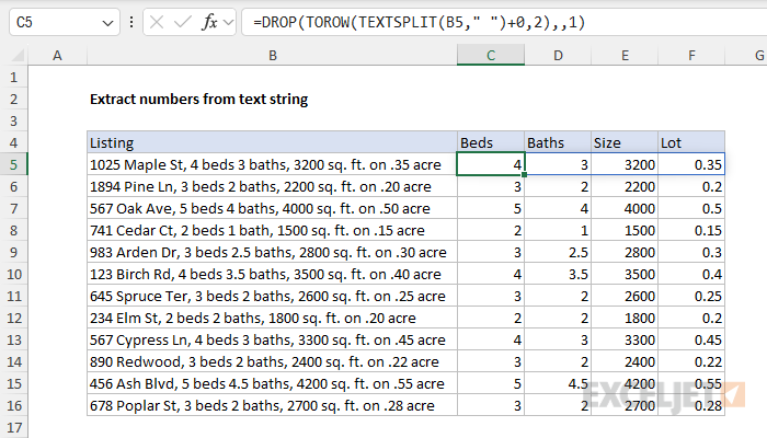
To extract numbers from a text string, you can use a clever formula based on the TEXTSPLIT and TOROW functions. In the worksheet shown, the formula in cell C5 is:
=DROP(TOROW(TEXTSPLIT(B5," ")+0,2),,1)
As the formula is copied down, it extracts the beds, baths, size, and lot information for each property listing. The numeric portion of the address function is discarded.
Generic formula
TOROW(TEXTSPLIT(A1," ")+0,2)
Explanation
In this example, the goal is to extract the numbers from a set of property listings which describe the number of bedrooms and bathrooms, the size of the house in sq. ft., and the size of the lot in acres. Traditionally, this kind of problem has been quite difficult in Excel because each number must be extracted with a separate, carefully configured formula (example). However, in the latest version of Excel, new functions like TEXTSPLIT, TOROW, and DROP make the process much easier.
The approach
The overall approach in the worksheet shown above is to split the text in column B into separate words, remove all non-numeric words with a clever hack, and remove the first number, which represents the street number. The formula in cell C5, copied down, looks like this:
=DROP(TOROW(TEXTSPLIT(B5," ")+0,2),,1)
Working from the inside out, the first step is to split the text string into separate words.
Splitting text into words
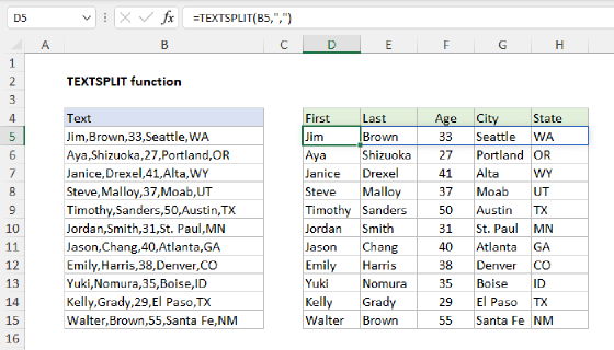
To split the text strings in column B into separate words, we use the TEXTSPLIT function. TEXTSPLIT is a flexible function that can be configured with up to six arguments, but in this case, we need just two: text and column delimiter:
TEXTSPLIT(B5," ") // split text into words
For text, we provide cell B5. For col_delimiter, we provide a single space (" "). With these inputs, TEXTSPLIT splits the text at each space and returns an array like this:
{"1025","Maple","St,","4","beds","3","baths,","3200","sq.","ft.","on",".35","acre"}
Note that all values at this point are text strings, which Excel encloses in double quotes ("").
Removing the non-numeric values
The next step in the process is to remove the non-numeric values. At first glance, this is a puzzle, because all the values in the array are text, including the numbers. This is one of those cases where the easiest solution is a hack that depends on knowing how the Excel formula engine works. Briefly, Excel tries to convert a text string to a number when it is involved in a math operation. For example, if we add 1 to a true number and a number that is text, it works in both cases:
=100+1 // returns 101
="100"+1 // returns 101
This happens because Excel silently converts the text "100" into the number 100 and then proceeds with the addition. However, if we try to add a number to a text string that can't be converted to a number, the operation fails with a #VALUE! error:
="apple"+1 // returns #VALUE!
It turns out that we can use this behavior in this problem to easily remove the non-numeric values. First, we add zero to the result from TEXTSPLIT:
TEXTSPLIT(B5," ")+0
As explained above, Excel will try to convert the text values returned by TEXTSPLIT into numbers. The result is an array like this:
{1025,#VALUE!,#VALUE!,4,#VALUE!,3,#VALUE!,3200,#VALUE!,#VALUE!,#VALUE!,0.35,#VALUE!}
Notice #VALUE! errors have replaced the non-numeric text values, while the numbers have survived the operation and are now true numeric values. In other words, we have forced all text values to errors and converted text to numbers at the same time. Next, we need to discard the errors. While we could use the FILTER function for this job, a simpler option is to use the TOROW function like this:
TOROW(TEXTSPLIT(B5," ")+0,2)
The purpose of TOROW is to transform an array into a single row. In this case, we already have a row, so we only use the TOROW function to remove errors by setting the ignore argument to 2. The result from this operation is a much cleaner array like this:
{1025,4,3,3200,0.35}
With ignore set to 2, TOROW removes the errors and leaves the numbers. Pretty cool, huh?
Removing the street number
The last step in this problem is to remove the first number from the final result, which is a street number, and a characteristic of the property itself. We can do this with the DROP function, which is designed to remove rows or columns from an array. In this case, since we have already split the text into separate columns, we want to remove the first column. We can do that by providing the number 1 for the columns argument:
=DROP({1025,4,3,3200,0.35},,1)
Notice the rows argument is left empty. The final result is an array with four numbers like this:
{4,3,3200,0.35}
This array spills into the range C5:F5. As the formula is copied down, the formula extracts the same information from each property as shown.
With the FILTER function
Just for the record, here is what a formula based on FILTER would look like, instead of TOROW:
=DROP(FILTER(TEXTSPLIT(B5," ")+0,ISNUMBER(TEXTSPLIT(B5," ")+0),2),,1)
The basic mechanics are the same. TEXTSPLIT creates an array of values, and adding zero forces the text values to errors, leaving numbers. The FILTER function then removes the errors by testing for numbers with the ISNUMBER function. However, because of the structure of FILTER, we need to repeat the TEXTSPLIT operation twice. The TOCOL solution avoids this redundancy, resulting in a compact, elegant formula.