TEXTSPLIT get numeric values

In this example, we have comma-separated text in column B. The goal is to split the text in column B into columns D through G while at the same time converting the numbers to true numeric values. The challenge is that TEXTSPLIT always returns text, so we need a way to convert the numbers while leaving the text values alone. 

The problem with TEXTSPLIT

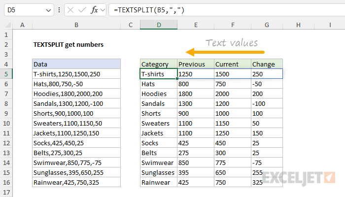
To split the text in column B into separate columns, we can use the TEXTSPLIT function with a simple formula like this:

TEXTSPLIT(B5,",")

This seems to work great. But the problem is that the numbers in columns E, F, and G aren't really numeric values. Instead, they are text values, as you can see by the way Excel aligns them to the left:

If you use a function like SUM to sum these numbers up, the result will be zero. How can convert these numbers as text to actual numeric values? Well, one option is to use the VALUE function.

Adding the VALUE function

The VALUE function is designed to convert text that appears in a recognized format (i.e. a number, date, or time format) into a numeric value. If we wrap the VALUE function around the TEXTSPLIT function, this is the result:

Notice the numbers in columns E, F, and G are now actually numeric values, as we can see by the way Excel right-aligns them. However, we now have a new problem — the VALUE function has corrupted the text values in column D. This happens because when VALUE tries to convert the text to a number, the operation fails with a #VALUE! error. What we need is a way to selectively convert the "numbers as text" to numbers while leaving the text values alone. We can do that with the IFERROR function.

Adding the IFERROR function

The IFERROR function returns a custom result when a formula generates an error, and a standard result when no error is detected. The syntax for IFERROR looks like this:

=IFERROR(value,value_if_error)

To illustrate how this works, we can start by adding IFERROR like this:

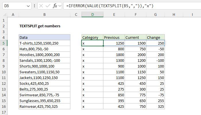
=IFERROR(VALUE(TEXTSPLIT(B5,",")),"x")

Notice we have simply embedded the original formula above into IFERROR as the value argument, then provided the value "x" for value_if_error. The result looks like this:

The "x" in column D tells us that IFERROR has encountered an error in this column, which is created when VALUE tries to convert the text values into numbers. The final step is to replace the "x" with the original text value. We can do that by simply repeating the original TEXTSPLIT formula. The final formula looks like this:

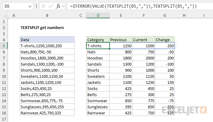
=IFERROR(VALUE(TEXTSPLIT(B5,",")),TEXTSPLIT(B5,","))

The result in the worksheet looks like this:

Optimizing with the LET function

The formula above works fine, but it would be inefficient with a large amount of data because we are running the same TEXTSPLIT operation twice. One way to improve performance is to use the LET function like this:

=LET(array,TEXTSPLIT(B5,","),IFERROR(VALUE(array),array))

In this formula, the result from TEXTSPLIT is assigned to a variable named "array". We then use array inside the IFERROR and VALUE functions as above. The key difference is that TEXTSPLIT runs just one time.