=TEXTSPLIT(text, col_delimiter, [row_delimiter], [ignore_empty], [match_mode], [pad_with])- text - The text string to split.
- col_delimiter - The character(s) to delimit columns.
- row_delimiter - [optional] The character(s) to delimit rows.
- ignore_empty - [optional] Ignore empty values. TRUE = ignore, FALSE = preserve. Default is FALSE.
- match_mode - [optional] Case-sensitivity. 0 = enabled, 1 = disabled. Default is 0.
- pad_with - [optional] Value to pad missing values in 2d arrays.
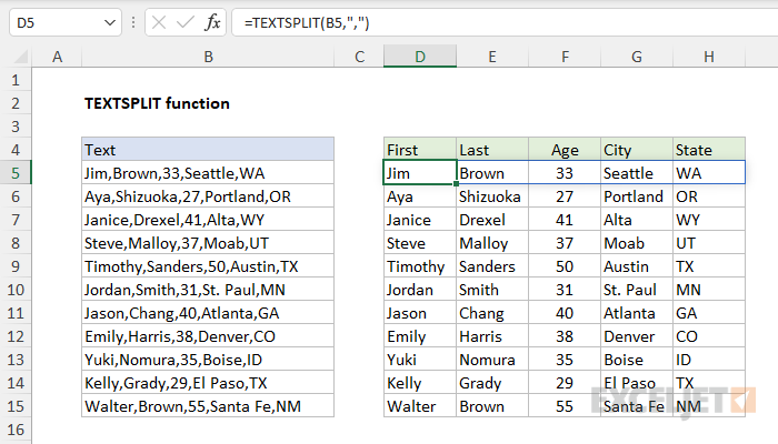
Using the TEXTSPLIT function
The TEXTSPLIT function splits a text string with a given delimiter into multiple values. The output from TEXTSPLIT is an array that will spill into multiple cells in the workbook.
Video: Excel TEXTSPLIT function
Split text into columns or rows
TEXTSPLIT can split a text string into columns or rows. To use TEXTSPLIT, you will need to provide the text to split and a delimiter. You can either provide a column delimiter (col_delimiter) to split text into columns, or a row delimiter (row_delimiter) to split text into rows. For example, the formula below splits the text "red-blue-green" into separate values in columns:
=TEXTSPLIT("red-blue-green","-") // returns {"red","blue","green"}
Note that the column delimiter is provided as a hyphen ("-). If we move the hyphen ("-") to the row delimiter position, the TEXTSPLIT function will return the same values split into rows:
=TEXTSPLIT("red-blue-green",,"-") // returns {"red";"blue";"green"}
Note that both formulas above return an array of three values and the only difference is the location of the delimiter. The values in this first array will spill into separate columns, and the values in the second formula will spill into rows. The example below shows how this looks on the worksheet:
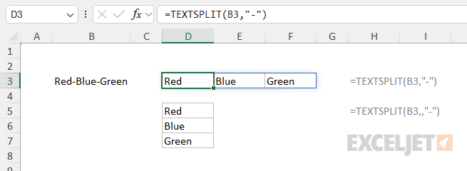
The first formula in cell D3 separates the three values into separate columns:
=TEXTSPLIT(B3,",") // returns {"Red","Blue","Green"}
The formula in cell D5 uses the same delimiter to split the text into separate rows:
=TEXTSPLIT(B3,,",") // returns {"Red";"Blue";"Green"}
In the second formula, the row_delimiter is left empty, and the same delimiter (",") appears as col_delimiter.
To summarize: provide a column delimiter if you want the results to be in separate columns and a row delimiter if you want the results to appear in separate rows.
TEXTSPLIT extracts all text separated by delimiters. Use TEXTBEFORE to extract text before a given delimiter, and TEXTAFTER to extract text after a given delimiter.
Behavior if no delimiter is found
If the provided delimiter is not found, TEXTSPLIT will return the original text unchanged. For example, if we use TEXTSPLIT on the text string "apple orange" with a period configured as the delimiter, TEXTSPLIT will return the original text:
=TEXTSPLIT("apple orange",".") // returns "apple orange"
The period (".") is not found, yet TEXTSPLIT behaves as if the delimiter was found at the end of the text. Both the TEXTBEFORE and TEXTAFTER functions have a similar feature, but it must be enabled with the match_end argument. With TEXTSPLIT, this behavior is automatic and useful.
Ignoring empty values
By default, TEXTSPLIT will include empty values in the text, where empty values are defined as two or more consecutive delimiters without a value in between. In practice, this means you will see empty cells in the worksheet when there is no value between delimiters, as you can see in the first formula below:
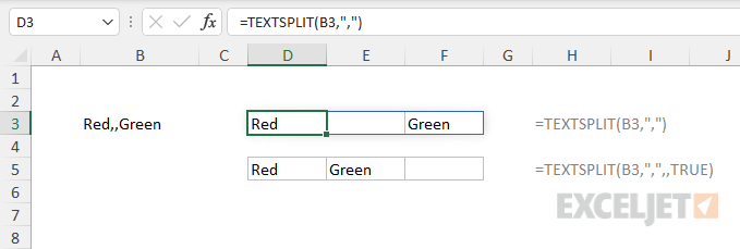
The formula in cell D3 does not include a value for ignore_empty, so empty values will appear:
=TEXTSPLIT(B3,",") // empty values will appear
To ignore (i.e., remove) empty values, set ignore_empty to TRUE, as in the second formula in cell D5:
=TEXTSPLIT(B3,",",,TRUE) // ignore empty values
In this case, TEXTSPLIT behaves as if the missing value does not exist at all. Only "Red" and "Green" are returned.
Note: you can use 1 and 0 in place of TRUE and FALSE for the ignore_empty argument.
Match mode
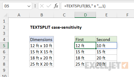
The fifth argument, match_mode, determines case sensitivity when looking for a delimiter. By default, TEXTSPLIT is case-sensitive and match_mode is zero (0). Supply 1 to disable case sensitivity. In the example below the delimiter is " x " and " X ". The formula in D5 sets match mode to 1 to make TEXTSPLIT ignore case. As a result, the formula works for both cases:
=TEXTSPLIT(B5," x ",,,1)
Rows and columns
TEXTSPLIT can split text into rows and columns at the same time, as seen below:
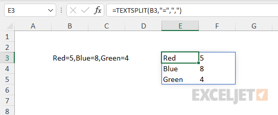
In this case, an equal sign ("=") is provided as col_delimiter and a comma (",") is provided as row_delimiter:
=TEXTSPLIT(B3,"=",",")
The resulting array from TEXTSPLIT contains 3 rows and 2 columns.
Padding
The last argument in TEXTSPLIT is pad_with. This argument is optional and will default to #N/A. Padding is used when the output contains rows and columns and a value is missing that would affect the structure of the array. In the worksheet below, "Blue" does not contain a quantity (there is no "=" delimiter). As a result, TEXTSPLIT returns #N/A where the quantity would go, to maintain the integrity of the array.
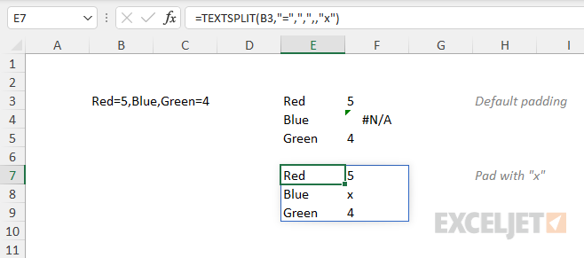
The formula in cell E3 contains does not specify a pad_with argument so the default value is returned:
=TEXTSPLIT(B3,"=",",") // default padding is #N/A
In cell E7, "x" is supplied for pad_with so "x" appears in cell F8 instead of #N/A.
=TEXTSPLIT(B3,"=",",",,"x")
Multiple delimiters
Multiple delimiters can be supplied to TEXTSPLIT as an array constant like {"x","y"} where x and y represent delimiters:
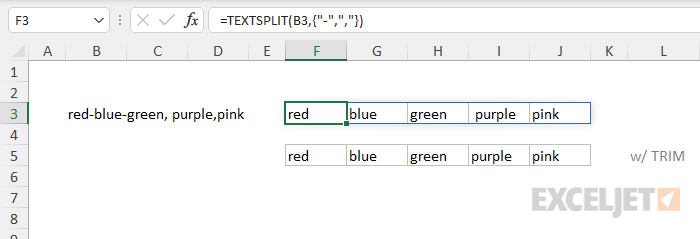
In the worksheet above, the text in B3 is delimited by both hyphens "-" and commas (","). The formula in cell F3 is:
=TEXTSPLIT(B3,{"-",","})
Notice also that there is an extra space separating green and purple. The TRIM function can be used to clean up extra space characters that appear in the output from TEXTSPLIT. The formula in F5 is:
=TRIM(TEXTSPLIT(B3,{"-",","}))
Notice the extra space that appears before purple in cell I3 is gone in cell I5.
Array of arrays
When using TEXTSPLIT, you might run into a limitation of the Excel formula engine where the formula will not return "arrays of arrays". When TEXTSPLIT is used on a single cell, it returns the text in a single array, and values spill onto the worksheet into multiple cells. However, when TEXTSPLIT is used on a range of cells, TEXTSPLIT returns an "array of arrays". The result may be a truncated version of the data or in some cases an error. Example here.