Get name from email address

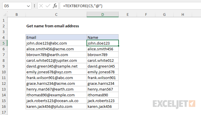
In this example, the goal is to extract the name from a list of email addresses. In the current version of Excel, the easiest way to do this is with the TEXTBEFORE function or the TEXTSPLIT function. In older versions of Excel, you can use a formula based on the LEFT and FIND functions. All three options are explained below.

TEXTBEFORE function

The TEXTBEFORE function returns the text that occurs before a given delimiter. The generic syntax for TEXTBEFORE supports many options:

=TEXTBEFORE(text,delimiter,[instance_num],[match_mode],[match_end],[if_not_found])

However, most of these arguments are optional. For this problem, we only need to provide the first two arguments, text and delimiter:

=TEXTBEFORE(text,delimiter)

Text is the text string to split, and delimiter is the location at which to split the string. Since all email addresses contain the "@" character separating the name from the domain, we can extract the name with a formula like this:

=TEXTBEFORE(C5,"@")

As the formula is copied down the column, it extracts the name from each of the emails as shown in the worksheet. For more details on TEXTBEFORE, see How to use the TEXTBEFORE function.

Note: You can use the TEXTAFTER function to extract the domain from the email.

TEXTSPLIT function

Another easy way to solve this problem is with the TEXTSPLIT function, which is designed to split a text string at a given delimiter and return all parts of the split string in a single step. To solve this problem with TEXTSPLIT, use a formula like this in cell D5:

=TEXTSPLIT(C5,"@")

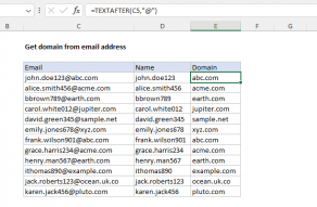
As the formula is copied down, TEXTSPLIT will split the email at the @ character and return the name and the domain. These two values will spill into column D and column E as seen below:

The advantage of this approach is that you get both the email and the domain with a single formula. For more details on TEXTSPLIT, see How to use the TEXTSPLIT function.

Legacy Excel

In older versions of Excel that do not provide the TEXTBEFORE  or TEXTSPLIT functions, you can use a formula based on the LEFT and FIND functions:

=LEFT(C5,FIND("@",C5)-1)

At the core, this formula extracts characters from the left with the LEFT function, using FIND to figure out how many characters to extract. C5 contains the email "john.doe123@abc.com", so FIND returns 12, since the "@" occurs as the 12th character. We then subtract 1 to prevent the formula from extracting the "@" along with the name:

FIND("@",C5)-1 // returns 11

The result is 11, which is returned directly to the LEFT function as the num_chars argument:

=LEFT(C5,11) // returns "john.doe123"

The final result returned by LEFT is "john.doe123". As the formula is copied down the column, it performs the same operation on each email address. Although this formula is more complicated than the TEXTBEFORE or TEXTSPLIT options above, it achieves the same result.