Explanation
In this example, the goal is to remove the protocol from a list of URLs. To remove the protocol from a URL, we need to remove the first part of the URL. Protocols typically look like this:
- http://
- https://
- sftp://
Notice that all protocols end with a double slash ("//"). In the current version of Excel, the easiest way to do this is with the TEXTAFTER function. In older versions of Excel, you can use a formula based on the MID and FIND functions. Both options are explained below.
TEXTAFTER function
The TEXTAFTER function returns the text that occurs after a given delimiter. TEXTAFTER supports many options, but for this problem, we only need to provide the first two arguments:
=TEXTAFTER(text,delimiter)
- Text: the text string to process.
- Delimiter: the place at which to split the text.
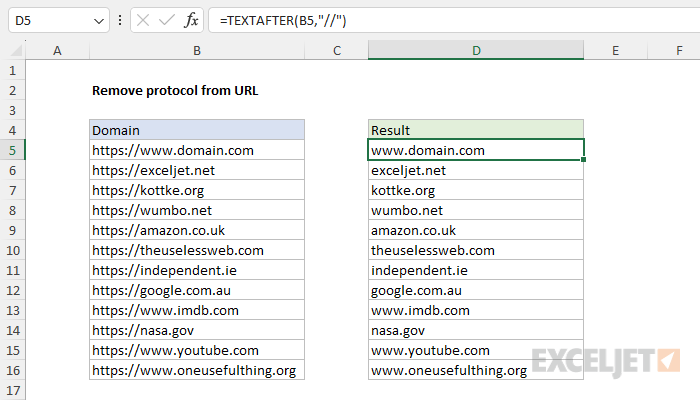
To remove all text up to and including the double slash, we can use the TEXTAFTER function like this:
=TEXTAFTER(B5,"//")
As the formula is copied down the table, it extracts the text that occurs after the double slash ("//"). The result is the original URL without the protocol.
Want to learn more about TEXTAFTER? Check out our guide: How to use the TEXTAFTER function.
Legacy Excel
In an older version of Excel without the TEXTAFTER function, you can remove the protocol from a URL with a formula based on the MID function and the FIND function like this:
=MID(B5,FIND("//",B5)+2,LEN(B5))
The core of this formula is the MID function, which extracts the text in a URL starting with the character after "//", and ending with the character before the trailing slash ("/"):
=MID(text,start_num,num_chars)
The text is the URL in cell B5. The start_num is calculated using the FIND function like this:
FIND("//",B5)+2
FIND returns the position of the double slash ("//") in the URL as a number. With the text "https://www.domain.com" in cell B5, FIND returns 9. We don't want to start extracting at character 9 however, we want to skip the double slash ("//") altogether, so we add 2 to the result from FIND which results in 11. This is the value used for start_num. At this point, we have:
=MID(B5,11,LEN(B5))
To provide a value for num_chars, we use the LEN function, which returns a count of all the characters in B5, which is 22. Using the LEN function like this is a shortcut, designed to simplify the formula. LEN will return 22, which is greater than the number of characters that remain. However, when num_chars exceeds the remaining string length, MID will simply extract all remaining characters. Using LEN to provide num_chars is an easy way to give MID a number that is always large enough, without the trouble of calculating exactly how many characters remain. Dropping in the value returned by the LEN function, we now have a formula that looks like this:
=MID(B5,11,22) // returns "www.domain.com"
The MID function begins extracting at character 11 and extracts all remaining text. The final result is "www.domain.com".


