Get domain from email address

In this example, the goal is to extract just the domain name from a list of email addresses. In the current version of Excel, the easiest way to do this is with the TEXTAFTER function or the TEXTSPLIT function. In older versions of Excel, you can use a formula based on the RIGHT, LEN, and FIND functions. All three options are explained below.

TEXTAFTER function

The TEXTAFTER function returns the text that occurs after a given delimiter. The generic syntax for TEXTAFTER supports quite a number of options:

=TEXTAFTER(text,delimiter,[instance_num],[match_mode],[match_end], [if_not_found])

However, most of the inputs are optional and for this problem, we only need to provide the first two arguments:

=TEXTAFTER(text,delimiter)

Here, text represents the text string to parse, and delimiter represents the place at which to begin extracting. Since all email addresses contain the @ character separating the name from the domain, we can extract the domain with a simple formula like this:

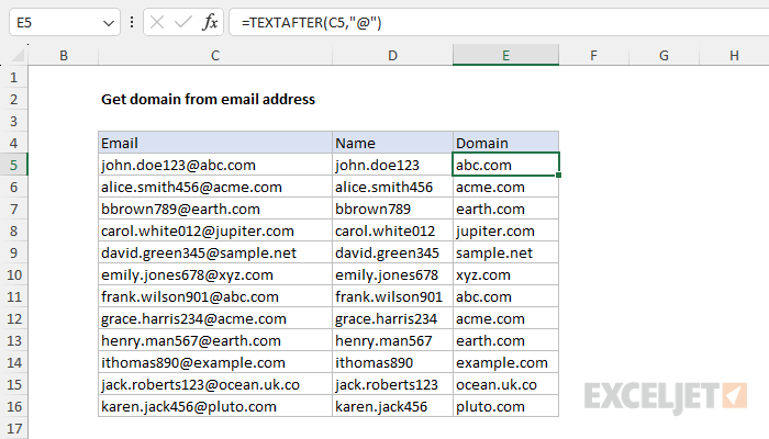
=TEXTAFTER(C5,"@")

As the formula is copied down the table, it extracts the domain name from each of the emails as shown in the worksheet. For more information, see How to use the TEXTAFTER function.

Note: You can use the TEXTBEFORE function to extract the name portion of the email.

TEXTSPLIT function

Another easy way to solve this problem is with the TEXTSPLIT function, which is designed to split a text string at a given delimiter and return all pieces of the string in a single step. To solve this problem with TEXTSPLIT, use a formula like this in cell D5:

=TEXTSPLIT(C5,"@")

As the formula is copied down, TEXTSPLIT will split the email at the @ character and return the name and the domain in one step:

The advantage of this approach is that you get both the email and the domain with a single formula. For more details on TEXTSPLIT, see How to use the TEXTSPLIT function.

Legacy Excel

In older versions of Excel that do not provide the TEXTAFTER  or TEXTSPLIT functions, you can use a formula based on the RIGHT, LEN, and FIND functions:

=RIGHT(C5,LEN(C5)-FIND("@",C5))

At the core, this formula extracts characters from the right with the RIGHT function, using FIND and LEN to figure out how many characters to extract. C5 contains the text "john.doe123@abc.com", so LEN returns 19 characters:

LEN(C5) // returns 19

FIND locates the "@" character inside the email address "john.doe123@abc.com". The "@" character is the 12th character, so FIND returns 12:

FIND("@",C5) // returns 12

Next, 12 is subtracted from 19, and the result (7) is returned directly to the RIGHT function as the num_chars argument. The RIGHT function then extracts 7 characters from the email address, starting from the right, and returns "abc.com" as a final result. The complete formula is evaluated like this:

=RIGHT(C5,LEN(C5)-FIND("@",C5))
=RIGHT(C5,19-12)
=RIGHT(C5,7) // returns "abc.com"

Although this formula is more complicated than the formulas based on TEXTAFTER or TEXTSPLIT, it will work just fine. If you get unexpected results, you might need to run the email addresses through the TRIM function to strip leading or trailing spaces, since trailing spaces will cause incorrect results. Once you have trimmed email addresses, apply the formula above.