Cell contains specific words

In this example, the goal is to test the text in a cell and return TRUE if it contains one or more specific words, and FALSE if not. Notice the emphasis here is on words, not substrings. For example, if we are testing for the word "green" and the text contains the word "evergreen" but not the word "green" the formula should return FALSE. Traditionally, this has been a difficult problem in Excel because there has not been a simple way to parse text into words. However, with the introduction of the TEXTSPLIT function, it is easy to split a text string directly into an array of words. Once we have the words in an array, they can be tested.

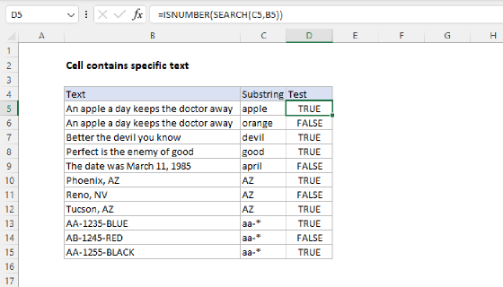
Note: The TEXTSPLIT function is only available in the most recent version of Excel. In older versions of Excel, you can use a similar formula that checks for a substring.

Table of Contents

• Using TEXTSPLIT to split text into words
• Testing for words
• Cell contains specific words
• Cell contains one of many words
• Cell contains at least 2 words
• Cell contains all words
• Cell contains some words but not others

Using TEXTSPLIT to split text into words

The TEXTSPLIT function is designed to split text into an array with a given delimiter. For example, in the formula below, we use TEXTSPLIT and a space (" ") as a delimiter to split the text "The sea is blue'' into 4 words:

=TEXTSPLIT("The sea is blue"," ") // returns {"The","sea","is","blue"}

Once we have the words in an array, we can do all kinds of things with them. We can count words, compare words, check for specific words, etc. TEXTSPLIT works very well for this task, but there is one complication you must be aware of: words are not always separated just by spaces. For example, what happens if we try the formula above on the text "The flag is red, reen, and blue":

=TEXTSPLIT("Red, green, and blue"," ")

In this case, the array returned by TEXTSPLIT looks like this:

{"Red,","green,","and","blue"}

Notice that the commas after "red" and "blue" are part of the output. This is bad. We don’t want punctuation to be included with the words, because it will cause problems later when we try to analyze the words. The solution is to expand the list of delimiters provided to TEXTSPLIT to include punctuation when needed. In this case, we simply need to add a comma (",") like this:

=TEXTSPLIT("Red,green, and blue",{","," "})

Note: we provide both the comma and the space using an array constant like {","," "}, which is a convenient way to supply more than one hard-coded value at the same time.

Now we are asking TEXTSPLIT to split words separated by a comma (",") and a space (" "). This works fine, but notice the result now contains an extra empty string as the third item in the array:

{"Red","green","","and","blue"}

This happens because TEXTSPLIT now splits the text at both delimiters. This is also bad, although, depending on the use case, it may not matter. Either way, we can easily remove the empty values by setting ignore_empty to 1:

=TEXTSPLIT("Red,green, and blue",{","," "},,1)

Notice we need to skip over and omit the row_delimiter argument. The revised formula now gives us the result we want, an array that contains four words without any punctuation or empty values:

{"Red","green","and","blue"}

Note: you will need to adjust the delimiters provided to TEXTSPLIT to suit the text you are working with.

We now have the core process we need to begin testing a cell for specific words.

Testing for words

Now that we have an array of words, the next step in this process is to check those words against our word(s) of interest. In the worksheet shown, we are looking for the word "green". There are different ways to go about this in Excel. For example, we could count instances of the word "green" in the array returned by TEXTSPLIT. However, a more scalable approach is to use the XMATCH function to check the result from TEXTSPLIT.

XMATCH is an upgrade to the MATCH function, and it returns the numeric location of a lookup value in an array of data. One nice feature of XMATCH is that it automatically performs an exact match, which is what we want in this case. To use XMATCH to look for "green" in the output from TEXTSPLIT, we use a formula like this:

XMATCH("green",TEXTSPLIT("Red, green, and blue",{".",", "," "}))

Notice we are using TEXTSPLIT as explained above, but we have embedded the TEXTSPLIT function inside the XMATCH function as the lookup array, with "green" as the lookup value.

XMATCH("green",TEXTSPLIT(B5,{".",","," "},,1)) 

After TEXTSPLIT runs, we have the following:

=XMATCH("green",{"Red","green","and","blue"}) // returns 2

Because "green" appears as the second value in the array returned by TEXTSPLIT, the XMATCH function returns 2 as a result. What happens if we check for a non-existent value, for example, the word "pink"? In that case, XMATCH returns an #N/A error:

=XMATCH("pink",{"Red","green","and","blue"}) // returns #N/A

To recap: when XMATCH finds a value, it will return a numeric position. When XMATCH does not find a value, it will return an #N/A error. At this point, we have a basic mechanism in place to check for a specific word in a cell. The only remaining task is to return TRUE or FALSE. The simplest way to do this is to use the ISNUMBER function like this:

=ISNUMBER(XMATCH("green",{"Red","green","and","blue"})) // returns TRUE
=ISNUMBER(XMATCH("pink",{"Red","green","and","blue"})) // returns FALSE

This works fine, but a more general approach, which will scale better to handle other related problems, is to use the COUNT function like this:

=COUNT(XMATCH("green",{"Red","green","and","blue"})) // returns 1
=COUNT(XMATCH("pink",{"Red","green","and","blue"})) // returns 0

The COUNT function only counts numeric values. So, when XMATCH returns a number, COUNT will return a positive number. When XMATCH returns an error, COUNT will return zero. To get a TRUE or FALSE result we can check to see if the count is greater than zero.

=COUNT(XMATCH("green",{"Red","green","and","blue"}))>0 // TRUE
=COUNT(XMATCH("pink",{"Red","green","and","blue"}))>0 // FALSE

We now have all the pieces we need to test for specific words in a cell.

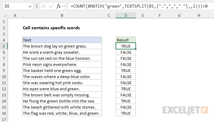
Cell contains specific words

Returning to the example shown in the worksheet above, the goal is to test for a given word and return TRUE or FALSE. This is accomplished by a formula like this in cell D5:

=COUNT(XMATCH("green",TEXTSPLIT(B5,{".",","," "},,1)))>0

Working from the inside out, TEXTSPLIT is configured to split the text in cell B5 using three delimiters supplied in an array constant like this:

TEXTSPLIT(B5,{".",", "," "},,1)

• text - cell B5
• col_delimiter - {".",","," "}
• row_delimiter - omitted
• ignore_empty - 1 (equivalent to TRUE)

Note that we provide three separate delimiters: a period ("."), a comma (",") and a space (" "). We also set ignore_empty to TRUE by providing 1. This is an important detail. We want TEXTSPLIT to ignore empty values because the delimiters will sometimes split text in a way that results in empty strings (""). Enabling the ignore empty behavior will remove any empty values that creep into the output from TEXTSPLIT.

In cell D5, the result from TEXTSPLIT is an array of seven words like this:

{"The","brown","dog","lay","on","green","grass"}

Next, since "green" appears as the sixth word, the XMATCH function returns 6, COUNT returns 1, and the final result is TRUE:

=COUNT(XMATCH("green",{"The","brown","dog","lay","on","green","grass"}))>0
=COUNT(2)>0
=1>0
=TRUE

Note: XMATCH is not case-sensitive, so testing for "Green" or "green" will return the same result.

Cell contains one of many words

Another common challenge is to test a cell for one of many words, as seen in the worksheet below. Here, the goal is to test text values in column B to see if they contain any one of the three words that appear in the range F5:F7, which is named "words".

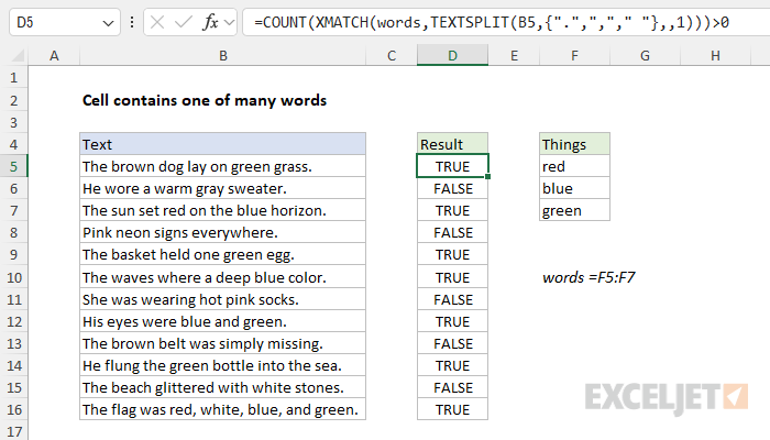
How should we adjust the formula to handle more than one lookup value? As it turns out, we can use the same formula we used above, replacing the text "green" with the named range words (F5:F7):

=COUNT(XMATCH(words,TEXTSPLIT(B5,{".",","," "},,1)))>0

The difference is that the named range words contains three words, which Excel represents in an array like this:

{"red";"blue";"green"}

Note: The named range is optional but provides some nice conveniences: it automatically behaves like an absolute reference and it makes the formula more readable. If you prefer, you can use a regular absolute reference ($F$5:$F$7) instead.

Because we are now giving XMATCH three separate lookup values, it will return 3 results like this:

{#N/A;#N/A;6}

The first #N/A error tells us that "red" was not found. The second #N/A error indicates that "blue" was not found. The last result, 6, tells us that the word "green" appeared as the sixth word in the array returned by TEXTSPLIT. The COUNT function only counts numbers so it returns 1 and the final result is TRUE. You can increase or decrease the number of words provided to XMATCH and the formula will continue to work correctly.

Note: this formula will return TRUE if any number of words is found.

Cell contains at least 2 words

Now that we have the basic formula working, we can easily adjust the logic to suit more specific use cases. For example, we can require the cell to contain at least 2 of the words provided, as seen in the screen below:

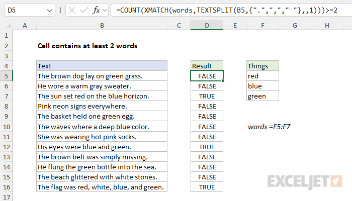
In this worksheet, the formula in cell D5 now looks like this:

=COUNT(XMATCH(words,TEXTSPLIT(B5,{".",","," "},,1)))>=2

Notice that this formula is almost exactly the same as the formula above. The only difference is that we are checking the result from COUNT with >=2, to require that there be at least two matching words in cell B5. In cell B5, the result is FALSE because only the word "red" is found in the text, as explained above. However, in cell D7, the result is TRUE, since both "red" and "blue" appear in cell B7, so COUNT returns 2. The formula in cell B7 evaluates like this:

=COUNT(XMATCH(words,TEXTSPLIT(B7,{".",","," "},,1)))>=2
=COUNT({4;7;#N/A})>=2
=2>=2
=TRUE

Cell contains all words

How can we adjust the formula to require that all given words appear in a cell? This can be done with another small adjustment, as seen in the worksheet below:

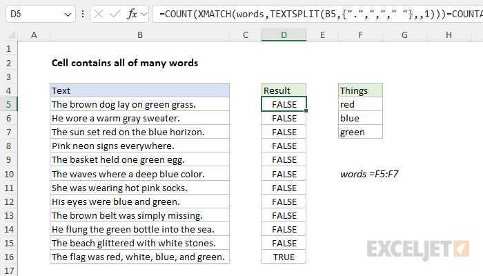
The formula in cell D5, copied down, looks now like this:

=COUNT(XMATCH(words,TEXTSPLIT(B5,{".",","," "},,1)))=COUNTA(words)

In this formula, we compare the count of "hits" returned by COUNT to the count of words returned by the COUNTA function. When the counts are equal, it means we found all given words in the text and the formula returns TRUE. When the counts are not equal, it means at least 1 word wasn't found and the formula returns FALSE. We use COUNTA to count the words because COUNTA will count both numbers and text values.

Cell contains some words but not others

As a last example, let's look at how to test a cell for certain specific words while at the same time specifically excluding others. This is the behavior we want:

1. If a cell contains specific words of interest and does not contain other specific words, the result should be TRUE
2. If a cell contains specific words of interest and does contain other specific words, the result should be FALSE

This makes the problem a bit more challenging, but we can still use the same approach described above. To make the formula more efficient and easier to read, we'll add the LET function to the mix. LET will enable us to parse the source text into words just one time and store the result in a variable where it can be reused.

In the worksheet below, we are testing the text in column B for the words "red", "blue", and "green" while at the same time excluding cells that contain the words "pink" or "brown":

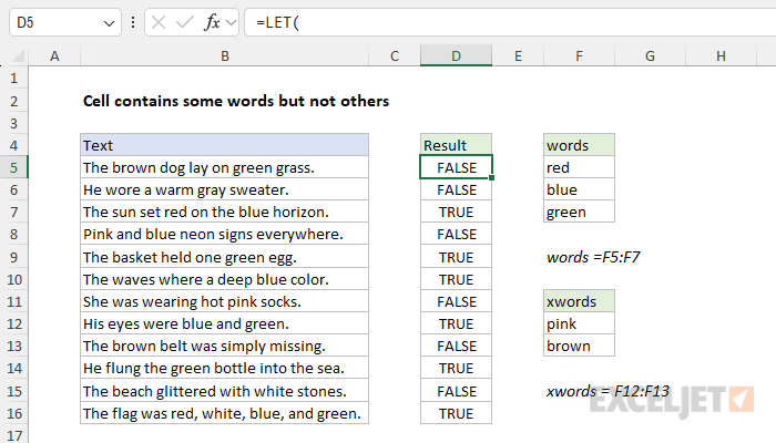
Notice that we have also added a named range to the worksheet: The range F5:F7 is named "words" as before and the range F12:F13 is now named "xwords". The idea is that xwords contains words that we want to exclude. The formula in cell D5 looks like this:

=LET(
  source,TEXTSPLIT(B5,{".",","," "},,1),
  AND(
    COUNT(XMATCH(words,source))>0,
    COUNT(XMATCH(xwords,source))=0)
)

In the first line of the formula, we use TEXTSPLIT as described above to create an array of words from the text in cell B5, which is assigned to a variable called "source":

source,TEXTSPLIT(B5,{".",","," "},,1),

Next, we use the AND function to check the results of two expressions. The first expression checks that we have at least one word of interest in the cell:

COUNT(XMATCH(words,source))>0

The second expression checks that we have zero words not of interest in the cell:

COUNT(XMATCH(xwords,source))=0)

The AND function will only return TRUE when both of the expressions above return TRUE. If either expression is FALSE, the result will be FALSE. This accomplishes our goal: the formula will return TRUE only when at least one word from words is found and zero words from xwords are found.