Cell ends with

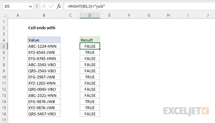
In this example, the goal is to test values in column B to see if they end with a specific text string, which is "jwb" in the worksheet shown. This problem can be solved with the RIGHT function, as explained below.

RIGHT function

The RIGHT function extracts a given number of characters from the right side of a text string. For example, the formula below returns the last three letters of "apple", which is "ple":

=RIGHT("apple",3) // returns "ple"

This means we can use the RIGHT function to test if cell B5 ends with "jwb" like this:

=RIGHT(B5,3)="jwb"

The RIGHT function extracts the last 3 characters in cell B5 and the result is compared to the string "jwb", forcing a TRUE or FALSE result. The formula is solved like this:

=RIGHT(B5,3)="jwb"
=RIGHT("ABC-1224-HNN",3)="jwb"
="HNN"="jwb"
=FALSE

For cell B5 the result is FALSE, since "ABC-1224-HNN" does not end with "jwb". In cell B6, however, the result is TRUE, since "XYZ-6543-JWB" does end with "jwb".

=RIGHT(B6,3)="jwb"
=RIGHT("XYZ-6543-JWB",3)="jwb"
="XYZ"="jwb"
=TRUE

Note that Excel is not case-sensitive by default, so "JWB"="jwb" will return TRUE in a formula. Also note the num_chars argument is set to 3 above because we want to work with the last 3 letters in the cell only. However, this value needs to be modified to suit the situation. For example, to test for a value that ends with "apple", num_chars should be set to 5:

=RIGHT(B5,5)="apple"

Case-sensitive option

Excel is not case-sensitive by default, but you can easily adapt the formula to use the EXACT function to make the formula case-sensitive like this:

=EXACT(RIGHT(B5,3),"JWB")

EXACT takes two arguments, text1 and text2. EXACT will only return TRUE when text1 and text2 are exactly the same, taking into account case. For example:

=EXACT("abc","ABC") // returns FALSE
=EXACT("abc","Abc") // returns FALSE
=EXACT("abc","abc") // returns TRUE

Turning back to cell B6 in the worksheet shown, the two formulas below return different results:

=EXACT(RIGHT(B6,3),"jwb")// returns FALSE
=EXACT(RIGHT(B6,3),"JWB") // returns TRUE

The first formula returns FALSE because the EXACT function is case-sensitive, so "JWB" does not equal "jwb". The second formula returns TRUE because "JWB" does equal "JWB" taking into account case. Note that we don't need the equal to operator (=) in this formula because EXACT performs a comparison automatically.

If cell ends with

To adapt the formulas above to "If cell ends with", simply drop the formulas into the IF function as the logical test. For example, to return "Yes" when a cell ends with "jwb" and "No" when not, you can use a formula like this

=IF(RIGHT(B5,3)="jwb", "Yes", "No")

The case-sensitive version of the formula works the same way:

=IF(EXACT(RIGHT(B5,3),"JWB"), "Yes", "No")

Other functions

It is worth noting that Excel contains two other functions, the SEARCH function and the FIND function that are meant to look for a substring in a text value. They could be used to solve this problem, but they are more work to configure, so I don't see any advantage to using them. You could however use the COUNTIF function with a wildcard to solve this problem like this:

=COUNTIF(B5,"*jwb")<>0

This works fine, but keep in mind that COUNTIF is in a group of eight *IFS functions that won't accept an array for the range argument. This means you can't use COUNTIF to test values in an array returned by another operation. I don't like this limitation, so I avoid the *IFS functions when there is a good alternative.