Summary
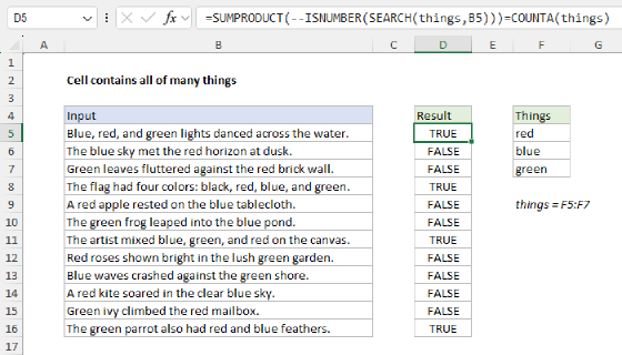
To test if a cell contains one of many strings, you can use a formula based on the SEARCH, ISNUMBER and SUMPRODUCT functions. The formula in C5, copied down, is:
=SUMPRODUCT(--ISNUMBER(SEARCH(things,B5)))>0
where things is the named range E5:E7.
Generic formula
=SUMPRODUCT(--ISNUMBER(SEARCH(things,A1)))>0
Explanation
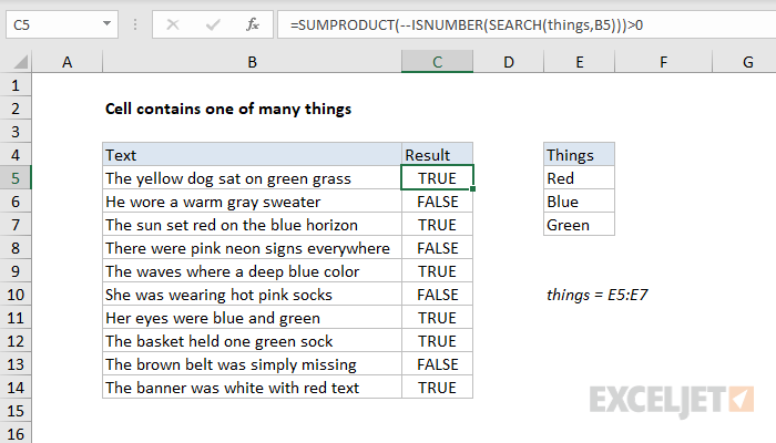
The goal of this example is to test each cell in B5:B14 to see if it contains any of the strings in the named range things (E5:E7). These strings can appear anywhere in the cell, so this is a literal "contains" problem. The formula in C5, copied down, is:
=SUMPRODUCT(--ISNUMBER(SEARCH(things,B5)))>0
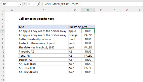
This formula is based on another formula that checks a cell for a single substring. If the cell contains the substring, the formula returns TRUE. If not, the formula returns FALSE:
ISNUMBER(SEARCH(substring,B5)) // test for substring
When the SEARCH function finds a string, it returns the position of that string as a number. If SEARCH doesn't find a string, it returns a #VALUE! error. This means ISNUMBER will return TRUE if there is a match and FALSE if not.
In this example, the goal is to check for more than one string, so we are giving the SEARCH function a list of strings in the named range things. Since there are 3 strings in things ("red", "green", and "blue"), SEARCH returns 3 results in an array like this:
{#VALUE!;#VALUE!;23}
Because "red" and "blue" aren't found , the SEARCH returns a #VALUE! error. However, because "green" appears near the end of the text in cell B5, SEARCH returns 23 (i.e. "green" begins at the 23rd character).
This array is returned directly to the ISNUMBER function, which converts the items in the array to either TRUE or FALSE:
ISNUMBER({#VALUE!;#VALUE!;23}) // returns {FALSE;FALSE;TRUE}
Logically, if we have even one TRUE in the array, we know a cell contains at least one of the strings we're looking for. The easiest way to check for TRUE is to add all values together. We can do that with the SUMPRODUCT function, but first we need to coerce the TRUE / FALSE values to 1s and 0s with a double negative (--) like this:
--{FALSE;FALSE;TRUE} // coerce to 1s and 0s
This yields a new array containing only 1s and 0s:
{0;0;1}
which is delivered directly to SUMPRODUCT:
=SUMPRODUCT({0;0;1}) // returns 1
With just one array to process, SUMPRODUCT sums the items in the array and returns a result. Any non-zero result means we have a "hit", so we add >0 to force a final result of TRUE or FALSE:
=SUMPRODUCT({0;0;1})>0 // returns TRUE
Note that any combination of matches will return a number greater than zero and cause the formula to return TRUE.
With a hard-coded list
It's not necessary to use a range for the list of strings to look for. You can also use an array constant. For example, to check for "red", "blue", or "green", you can use a formula like this:
=SUMPRODUCT(--ISNUMBER(SEARCH({"red","blue","green"},B5)))>0
SUM function
Historically, SUMPRODUCT often appears in array formulas, because it can handle arrays natively, without control + shift + enter. This makes the formula "more friendly" to most users. In Excel 365, which handles arrays natively, the SUM function can be used instead of SUMPRODUCT without control + shift + enter:
=SUM(--ISNUMBER(SEARCH(things,A1)))>0
Preventing false matches
One problem with this approach is you may get false matches from substrings that appear inside longer words. For example, if you try to match "dr" you may also find "Andrea", "drink", "dry", etc. since "dr" appears inside these words. This happens because SEARCH automatically does a "contains" match. For a quick hack, you can add space around the search words (i.e. " dr ", or "dr ") to avoid catching "dr" in another word. But this will fail if "dr" appears first or last in a cell, or appears with punctuation. If you need a more accurate solution, one option is to normalize the text first in a helper column, taking care to also add a leading and trailing space. Then you use the formula on this page on the resulting text.
Note: in the latest version of Excel, the TEXTSPLIT function provides a better way to search for specific words without catching unrelated substrings.