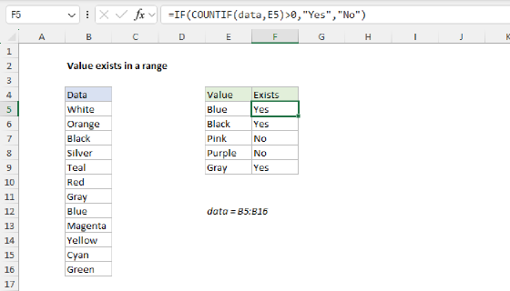
Summary
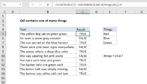
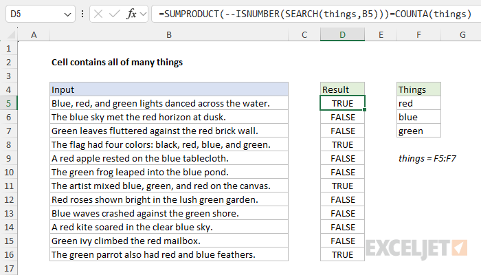
To test if a cell contains all of many values, you can use a formula based on the SEARCH function, with help from ISNUMBER, SUMPRODUCT, and COUNTA. In the worksheet shown, the formula in cell D5 is:
=SUMPRODUCT(--ISNUMBER(SEARCH(things,B5)))=COUNTA(things)
where things is the named range F5:F7. As the formula is copied down, it returns TRUE if the text in column B contains "red", "blue", and "green" and FALSE if not. The values to search for can be customized as needed.
Generic formula
=SUMPRODUCT(--ISNUMBER(SEARCH(things,A1)))=COUNTA(things)
Explanation
In this example, the goal is to build a formula that will return TRUE if a given cell contains all values that appear in a given range. We could build a formula that uses nested IF statements to check for each value, but that won't scale well if we have a lot of values to test because each new value will require another nested IF. The article below explains a more scalable approach based on the SEARCH function. For convenience, the values we are testing for are in the named range "things" which is F5:F7. The formula in cell D5 looks like this:
=SUMPRODUCT(--ISNUMBER(SEARCH(things,B5)))=COUNTA(things)
At a high level, this formula counts the matches found in cell B5 for the three values in things (F5:F7). Then it compares the count of matches found with the count of values in things. If the counts match, the formula returns TRUE. Otherwise, the formula returns FALSE. Working from the inside out, the core of the formula is this snippet based on the SEARCH function and the ISNUMBER function:
ISNUMBER(SEARCH(things,B5)
This code is based on a fairly common pattern in Excel formulas (explained in detail here) that are designed to test a cell for a specific text. The more generic version of the formula looks like this:
ISNUMBER(SEARCH(substring,text)
In a nutshell, the SEARCH function searches text for a substring. If the substring is found, SEARCH returns the location of the match as a number. If the substring is not found, SEARCH returns a #VALUE error. The ISNUMBER function is used to convert the result from SEARCH into TRUE or FALSE.
The twist in this formula is that we are not searching for a single substring. Instead, we are searching for 3 different substrings in the named range things (F5:F7). Because we are giving SEARCH three different substrings to look for, SEARCH will return three separate results in an array. In cell B5, the results from SEARCH look like this:
{7;1;16}
These numbers represent the location of "red", "blue", and "green" in the text from cell B5. The text "red" begins at character 7, "blue" begins at character 1, and "green" begins at character 16. These locations are delivered to the ISNUMBER function, which converts the results to TRUE or FALSE values. Because all three results are numbers, ISNUMBER returns an array that contains three TRUE values:
=ISNUMBER(SEARCH(things,B5))
=ISNUMBER({7;1;16))
={TRUE;TRUE;TRUE}
Next, we convert the TRUE / FALSE values to 1s and 0s with a double negative (--) operation:
--{TRUE;TRUE;TRUE}
The result is an array like this:
{1;1;1}
We take this step because we want to work with TRUE and FALSE like the numbers 1 and 0. Next, we process this array with SUMPRODUCT, which will give us a total count of matches:
=SUMPRODUCT({1;1;1}) // returns 3
The final step in the formula is to compare this result to the count of values in the named range things (F5:F7). To get a count of the values in things, we use the COUNTA function, which is designed to count both numbers and text:
=COUNTA(things)
=COUNTA({"red";"blue";"green"})
=3
If the counts are equal, the formula will return TRUE:
=SUMPRODUCT({1;1;1})=COUNTA(things)
=3=3
=TRUE
With a hard-coded list
There's no requirement to use a range for your list of things. If you're only looking for a small number of things, you can use a list in array format, called an array constant. For example, if you're just looking for the colors red, blue, and green, you can use {"red","blue","green"} and hardcode a count of values like this:
=SUMPRODUCT(--ISNUMBER(SEARCH({"yellow","green","dog"},B5)))=3
Simplifying the formula
There is a fair bit of complexity in computing a count of the substrings found, which involves ISNUMBER, a double negative (--) operation, and SUMPRODUCT. You might wonder why you can't just do this:
=COUNT(SEARCH(things,B5))=COUNTA(things)
The COUNT function only counts numeric values, so it should work, right? The answer is that it will work fine in Excel 2021 or later. But keep in mind that if the formula is opened in an older version of Excel, Excel will convert it to an array formula automatically. Then, if a user edits the formula and enters it again, without using control + shift + enter, it will break. The SUMPRODUCT approach is a workaround that ensures the formula will run cleanly in all versions of Excel without special handling. You can read more about this topic here: Why SUMPRODUCT?