Summary
To categorize text using keywords, you can use a formula based on the XLOOKUP function and the SEARCH function. In the example shown, the formula in C5 is:
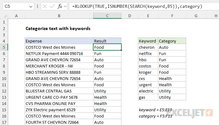
=XLOOKUP(TRUE,ISNUMBER(SEARCH(keyword,B5)),category)
where keyword (E5:E13) and category (F5:F13) are named ranges. As the formula is copied down, it searches the text in column B for a matching keyword in E5:E13 and returns the associated category from F5:F13. If no keyword is found, the formula returns a #N/A error. Notice the formula automatically performs a "contains" type match and is not case-sensitive.
Generic formula
=XLOOKUP(TRUE,ISNUMBER(SEARCH(keyword,A1)),category)
Explanation
In this example, the goal is to categorize various expenses using the categories shown in column F and the keywords shown in column E. This is a case where it seems like we should perform a lookup operation of some kind, but the problem is that the keywords appear embedded in the text and the structure is unpredictable. The article below explains two ways to solve this problem. The first approach, based on the XLOOKUP function is the simplest. The second approach, based on INDEX and MATCH is a more complicated array formula but will work in older versions of Excel without XLOOKUP. The keywords and categories are completely arbitrary and can be customized to suit the situation.
Note: For convenience, keyword (E5:E13) and category (F5:F13) are named ranges, but you can use absolute references or an Excel Table instead if you prefer.
Background study
This is a more advanced lookup formula. If you need a good introduction to XLOOKUP or INDEX and MATCH, these are good resources:
XLOOKUP solution
In the worksheet shown above, the formula in cell C5, copied down, looks like this:
=XLOOKUP(TRUE,ISNUMBER(SEARCH(keyword,B5)),category)
Working from the inside out, we first use the SEARCH function to look for keywords in cell B5 like this:
SEARCH(keyword,B5)
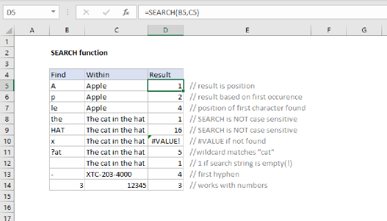
The SEARCH function returns the position of one text string inside another, and a #VALUE! error if the text string is not found. In this case, because the named range keyword contains 9 values:
SEARCH({"chevron";"netflix";"hbo";"costco";"kroger";"cvs";"urgent";"electric";"gas"},B5)
SEARCH returns an array that contains 9 results like this:
{#VALUE!;#VALUE!;#VALUE!;1;#VALUE!;#VALUE!;#VALUE!;#VALUE!;#VALUE!}
Notice all results are #VALUE! errors except for the fourth value, which is 1. This corresponds to the text "costco" appearing as the first word in the text in cell B5: "COSTCO West des Moines". Also, notice that SEARCH is not case-sensitive: it matches the lowercase "costco" in a text string that contains "COSTCO".
Next, the array above is returned to the ISNUMBER function, which converts the results into TRUE and FALSE values:
ISNUMBER({#VALUE!;#VALUE!;#VALUE!;1;#VALUE!;#VALUE!;#VALUE!;#VALUE!;#VALUE!})
ISNUMBER returns an array like this:
{FALSE;FALSE;FALSE;TRUE;FALSE;FALSE;FALSE;FALSE;FALSE}
The result from ISNUMBER is delivered directly to the XLOOKUP function as the lookup_array argument, and we can now simplify the original formula as follows:
=XLOOKUP(TRUE,{FALSE;FALSE;FALSE;TRUE;FALSE;FALSE;FALSE;FALSE;FALSE},category)
We can now finally see how the formula works. XLOOKUP is configured with the lookup_value set to TRUE. XLOOKUP locates the TRUE in the fourth position of the array returned by ISNUMBER and SEARCH, and returns the fourth item in category, "Food", as a final result. As the formula is copied down, the same operation is performed for each expense listed in column B.
For a more detailed explanation of the search method used in this formula see this example.
INDEX and MATCH solution
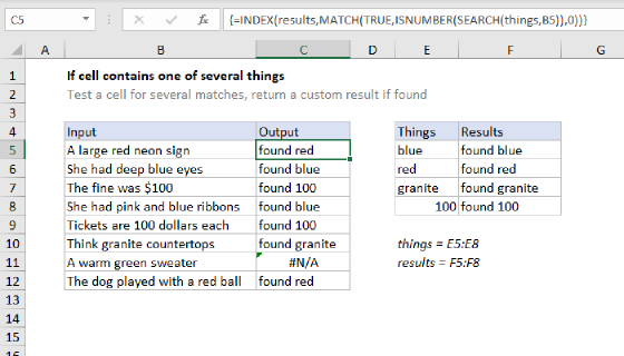
In older versions of Excel without the XLOOKUP function, you can use an alternative formula based on INDEX and MATCH. The equivalent formula in C5 looks like this:
=INDEX(category,MATCH(TRUE,ISNUMBER(SEARCH(keyword,B5)),0))
where keyword (E5:E13) and category (F5:F13) are named ranges.
Note: this is an array formula and must be entered with control + shift + enter in Excel 2019 and older. In Excel 2021 and newer, array formulas are native so the formula will "just work" without special handling.
The operation of this formula is similar to the XLOOKUP formula above. Inside the MATCH function, we use the SEARCH function to search cells in column B for every listed keyword in the named range keyword (E5:E13):
SEARCH(keyword,B5)
Because we are looking for multiple items (in the named range keyword), we'll get back multiple results like this:
{#VALUE!;#VALUE!;#VALUE!;1;#VALUE!;#VALUE!;#VALUE!;#VALUE!;#VALUE!}
The #VALUE! error occurs when SEARCH can't find the text. When SEARCH does find a match, it returns a number that corresponds to the position of the text inside the cell. To change these results into a more usable format, we use the ISNUMBER function, which converts all values to TRUE/FALSE like so:
{FALSE;FALSE;FALSE;TRUE;FALSE;FALSE;FALSE;FALSE;FALSE}
This array goes into the MATCH function as the lookup_array, with the lookup_value set to TRUE, and match_type set to 0 to force an exact match. MATCH returns the position of the first TRUE it finds in the array (4 in this case) which is provided to the INDEX function as the row_num:
=INDEX(category,4)
INDEX returns the 4th item in category, "Food", as a final result.
Preventing false matches
One problem with this approach is you may get false matches from substrings that appear inside longer words. For example, if you try to match "dr" you may also find "Andrea", "drink", "dry", etc. since "dr" appears inside these words. This happens because SEARCH looks for a substring and has no concept of words. For a quick hack, you can add space around the search words (i.e. " dr ", or "dr ") to avoid catching "dr" in another word. But this will fail if "dr" appears first or last in a cell, or appears with punctuation, etc. If you need a more accurate solution, one option is to normalize the text first in a helper column, taking care to also add a leading and trailing space. Then you can search for whole words surrounded by spaces.
In the latest version of Excel, another option is to use the TEXTSPLIT function with the XMATCH function like this:
=XLOOKUP(TRUE,ISNUMBER(XMATCH(keyword,TEXTSPLIT(B5,{".",", "," "}))),category)
In this formula, we have replaced the SEARCH function with XMATCH and TEXTSPLIT. The result is that we are splitting the text in B5 into an array of actual words, and then checking the words for keywords with XMATCH. For a detailed explanation of how this works, see this example.