Summary
There are eight widely used functions in Excel that use a syntax different from other functions in Excel. This syntax can make these functions more challenging to use, because it is not intuitive. Read on for important information about COUNTIF, COUNTIFS, SUMIF, SUMIFS, AVERAGEIF, AVERAGEIFS, MINIFS, and MAXIFS.
There are eight functions in Excel that work differently than you might realize. I call these "range-based conditional functions" or RACON (Ray-con) functions for short, because these functions apply criteria to a range and return a single result based on supplied criteria. In other words, these functions perform range-based, conditional aggregation. Here is the list of RACON functions:
| Function | Purpose |
|---|---|
| AVERAGEIF | Conditional average with one condition |
| AVERAGEIFS | Conditional average with one or more conditions |
| COUNTIF | Conditional count with one condition |
| COUNTIFS | Conditional count with one or more conditions |
| MINIFS | Conditional minimum with one or more conditions |
| MAXIFS | Conditional maximum with one or more conditions |
| SUMIF | Conditional sum with one condition |
| SUMIFS | Conditional sum with one or more conditions |
Click any function above for details and many examples.
Other Excel MVPs I know refer to this same group of functions as the *IFS functions.
What's different?
Although these functions are widely used, they operate differently in three key ways you may not have noticed:
- Logical expressions are split into two parts
- Ranges are required, you can't substitute arrays
- Other miscellaneous quirks
In the article below, I explain these differences in some detail.
Once you understand how these functions work, you can more easily get them to do what you want. In addition, you'll have a better idea about when you should explore alternatives.
Note: although the examples below deal exclusively with the COUNTIFS function, the same differences apply to all functions in the table above.
Logical expressions are split
A key difference in these functions versus others is that they apply criteria in a special way, by separating the logical expressions into two parts: range and criteria. For example, the basic syntax for COUNTIFS looks like this:
=COUNTIFS(range,criteria,range,criteria,etc)
I assume this was done for ease and convenience, to somehow make it "easier" to enter formula criteria without really understanding how to enter criteria as an expression, but it has consequences. For example, let's say you want to test the value in A1 and return TRUE when the value is greater than 5. With the IF function the syntax is simple:
=IF(A1>5,TRUE)
Nothing special, right? The logical expression, A1>5, makes perfect sense, and we can copy it down the column to test all values:
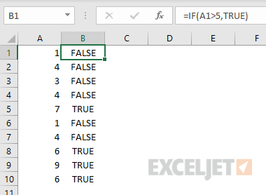
Note: I am embedding the expression A1>5 in the IF function only to illustrate how a logical expression would typically appear inside another function. The expression by itself (i.e. =A1>5), will create exactly the same TRUE/FALSE result.
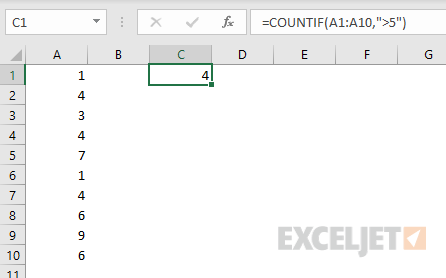
Now, let's say you want to count values in A1:A10 greater than 5 with the COUNTIFS function. This requires the following formula:
=COUNTIFS(A1:A10,">5")
Notice anything strange about this formula? What's that text (">5") doing in there?
Isn't 5 a numeric value? Yes, indeed.
This happens because the logical expression A1:A10>5 has been split into two parts. The range A1:A10 is perfectly valid, so it remains unquoted, but >5 is a partial and invalid expression. As a result, it must appear in quotes like ">5".
Somewhere behind the scenes, the Excel formula engine reassembles the text into a valid expression again:
A1:A10>5 // reassembled expression
Things get even weirder when we involve another cell in the criteria. For example, let's say we want to check values greater than B1. With the IF function, this is straightforward:
=IF(A1>B1,TRUE) // simple
But let's say we want to count values in A1:A10 that are greater than B1. Now we need to write:
=COUNTIFS(A1:A10,">"&B1) // what the ??
We are counting numeric values, but we need to use both concatenation and quoted text? Yes.
But note the cell reference itself is not quoted :)

What about text values? Suppose we want to check if a cell equals "apple". With IF, the logic is simple:
=IF(A1="apple",TRUE)
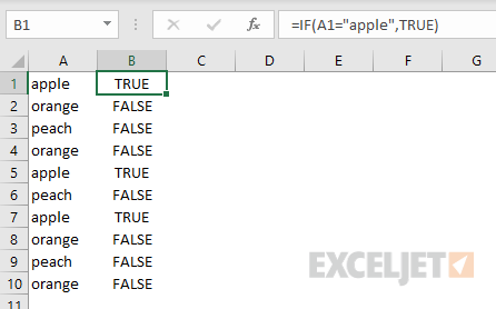
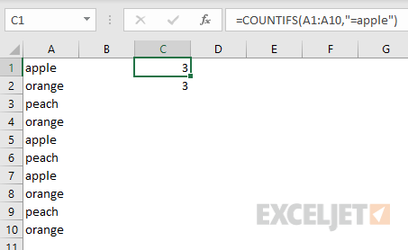
Now, what if we want to count cells equal to "apple"?
Both of these formulas will work:
=COUNTIFS(A1:A10,"=apple")
=COUNTIFS(A1:A10,"apple")
Basically, the "equals to" (=) operator is implied, so it's not required.
So, the logic is simpler, but quirky. In a similar way, you can count values equal to 5, with either:
=COUNTIFS(A1:A10,5) // no text
=COUNTIFS(A1:A10,"=5") // text
As above, both will work.
To summarize, because RACON functions split logical expressions into two parts, they require a unique syntax:
- Criteria that include logical operators must be enclosed in double quotes ("")
- The equals to (=) operator can be omitted (or not)
- Criteria based on another cell must use concatenation
Let's look next at the second key difference, ranges.
Ranges are required
A second key difference with RACON functions is range arguments. When a RACON function asks for a range, you must provide a range — you can't provide an in-memory array*.
This may not seem like a big deal at first. After all, the data is on the worksheet, right? So why not supply a range? However, in real-life situations, this requirement has consequences.
One example is dates. Let's say you want to check dates in A1:A10 to see which ones are in June?
With the IF function, you can simply use the MONTH function like this:
=IF(MONTH(A1)=6,TRUE) // month is 6?
The logic is simple: extract the month number with the MONTH function and compare the result to 6. If I put the formula in B1 and copy it down to B10, we'll get TRUE for dates in the month of June, and FALSE for all other dates:
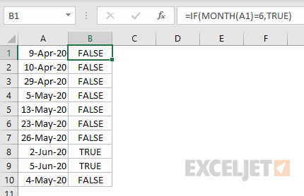
By the way, this is an example of nesting one formula inside another.
Now, how can we count the dates in A1:A10 that are in June? You might think we could use the MONTH function like we did with IF:
=COUNTIFS(MONTH(A1:A10),6) // nope
Nope. While this looks perfectly reasonable, it isn't going to work. Excel won't even let you enter the formula. Instead, it will throw a generic "There's a problem with this formula" error. In fact, the "problem" is that you must supply a range as the first argument to COUNTIFS.
Even though the MONTH function will happily give you all 10 month numbers in an array, an array won't cut it. You must supply a range.
Okay, so how can you get COUNTIFS to count dates in June? It's not pretty:
=COUNTIFS(A1:A10,">="&DATE(2020,6,1),A1:A10,"<="&DATE(2020,6,30))
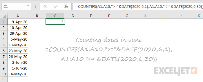
We are basically using the DATE function to hardcode start and end dates into the formula and using multiple criteria. The first condition tests for dates greater than or equal to June 1, the second condition tests for dates less than or equal to June 30.
If we put the date "1-June-2020" into another cell, B1, we can make things slightly less painful by using the EOMONTH function to calculate the last day in June:
=COUNTIFS(A1:A10,">="&B1,A1:A10,"<="&EOMONTH(B1,0))
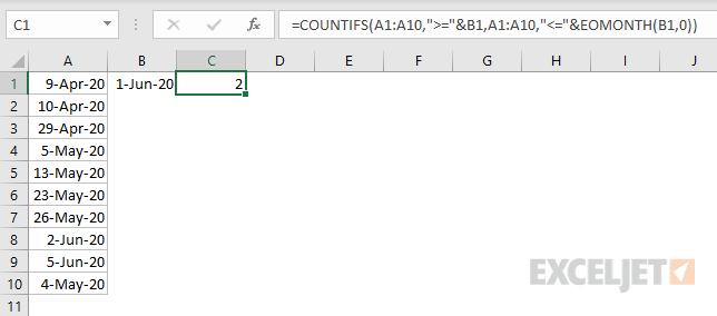
But we still can't avoid the monkey business of concatenation. And, I should note, both of the COUNTIFS examples above are testing for dates in June 2020, not just June.
The problem in a nutshell is that because COUNTIFS requires a range, we lose the power to manipulate values in that range directly.
** To be clear,* spill ranges work fine in RACON functions, since they are ranges on the worksheet.
Other quirks
RACON functions also have some other quirks, including:
- They strip leading zeros in text-based numbers
- They evaluate certain logical expressions differently
- They evaluate very long numbers differently
- 3D references are not allowed for range arguments
Alternatives
Now, how can we count dates in June with a function that doesn't have these limitations? Well, before the Dynamic Array version of Excel arrived, SUMPRODUCT would be the most streamlined solution:
=SUMPRODUCT(--(MONTH(A1:A10)=6))
This is an array formula, but it does not require control + shift + enter.
In the Dynamic Array version of Excel, we can use the SUM function in the same way:
=SUM(--(MONTH(A1:A10)=6))
This does require control + shift + enter in earlier versions of Excel, but in Dynamic Excel, it will just work.
Both formulas use the double-negative trick to change TRUE FALSE values to 1's and 0's, so they can be counted.
We can also use the FILTER function like this:
=COUNT(FILTER(A1:A10,MONTH(A1:A10)=6))
This involves one more function, but notice the logic used inside FILTER to test for month is exactly the same.
Consistency and the future
The beauty of the new functions in Excel is that they all use logical expressions in the same consistent way. Even better, dynamic arrays let you build simple array formulas with the same clean and simple syntax, no fancy keystrokes required.
Although the RACON functions are still useful and, in some slightly twisted way, "easier", many future Excel formulas will be simpler, more consistent, and easier to learn.


