Count long numbers

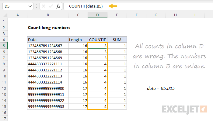
In this example the goal is to count numbers longer than 15 digits with a formula. The COUNTIF function may seem like this logical choice. However, if you try to count very long numbers (16+ digits) in a range with the COUNTIF function, you may see incorrect results, due to a bug in how RACON functions handle long numbers, even when the numbers are stored as text. You can see this problem in the worksheet below. All counts in column D are incorrect. Each number in column B is unique, yet the count returned by COUNTIF suggests the numbers are duplicates.

 =COUNTIF(data,B5)

This problem is related to how Excel handles numbers. Excel can only handle 15 significant digits, and if you enter a number with more than 15 digits in Excel, you will see the trailing digits silently converted to zero. The counting problem mentioned above arises from this limit.

Normally, you can avoid this limit by entering long numbers as text, either by starting the number with a single quote (i.e. '999999999999999999) or by formatting the cell(s) as Text before entering. As long as you don't need to perform math operations on a number, this is a good solution, and it will handle long numbers like credit card numbers and serial numbers without losing any numbers.

However, if you try to use COUNTIF to count a number with more than 15 digits (even when stored as text) you may see incorrect results. This happens because COUNTIF internally converts the text value back to a number at some point during processing, which triggers the 15 digit limit described above. With trailing digits converted to zero, long numbers may look like duplicates to RACON functions like COUNTIF, COUNTIFS, SUMIF, SUMIFS, etc. The solution is to use the SUM function or the SUMPRODUCT function, as explained below.

SUM function

One solution is to replace the COUNTIF formula with a formula that uses the SUM function. In the example shown, the formula in E5 is:

=SUM(--(data=B5))

The formula uses the named range data (B5:B9) and Boolean logic to count values. Working from the inside out, this expression compares all values in data (B5:B15) with the value in B5:

data=B5

Because data contains 11 cells, the result is an array of TRUE/FALSE results like this:

{TRUE;FALSE;FALSE;FALSE;FALSE;FALSE;FALSE;FALSE;FALSE;FALSE;FALSE}

Notice that the TRUE value corresponds to the first number in the range B5:B15, and all remaining values are FALSE. This tells us the number 1234567891234567 occurs just once in the data. Because the SUM function will ignore the logical values TRUE and FALSE, we use a double negative (--) to convert the TRUE and FALSE values to 1s and 0s:

--(data=B5) // returns {1;0;0;0;0;0;0;0;0;0;0}

This results in an array containing only 1s and 0s, which is returned directly to the SUM function:

=SUM({1;0;0;0;0;0;0;0;0;0;0}) // returns 1

The SUM function sums the items in the array and returns 1 as a final result.

Note: this formula must be entered with Control + Shift + Enter in Legacy Excel.

SUMPRODUCT function

In Legacy Excel, the formula above is an array formula and must be entered in a special way. To avoid this step, you can replace the SUM function with the SUMPRODUCT function like this:

=SUMPRODUCT(--(data=B5))

The behavior of the formula is the same, but because SUMPRODUCT is in a small group of functions that can handle array operations natively, the formula requires no special handling. For more on this topic, see Why SUMPRODUCT?