Summary
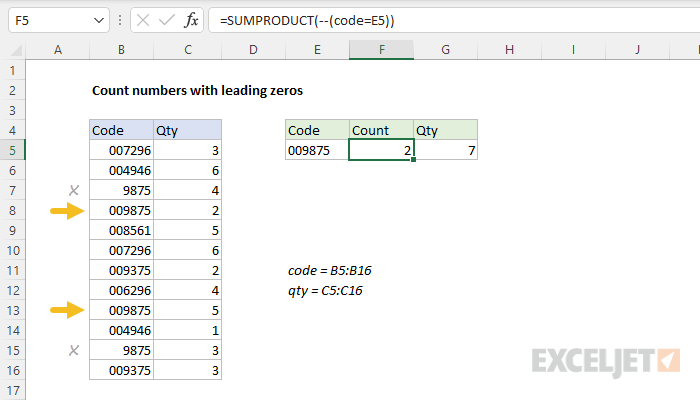
To count numbers that contain leading zeros, you can use the SUMPRODUCT function with a simple logical expression. In the example shown, the formula in cell F5 is:
=SUMPRODUCT(--(code=E5))
where code is the named range B5:B16.
Generic formula
=SUMPRODUCT(--(range=value))
Explanation
In this example, the goal is to count numbers that contain leading zeros. In cell E5, we have the code "009875" and we want to count how many times this code appears in the range B5:B16. The challenge is that Excel can be finicky with leading zeros. Technically, the values in B5:B16 are text, as is the value in E5. However, sometimes text values that contain numbers are converted to numeric values as they go through Excel's calculation engine. When this happens, the leading zeros will be silently removed, which can cause an incorrect result. The article below explains the problem in more detail. For convenience, code (B5:B16) and qty (C5:C16) are named ranges.
COUNTIF with leading zeros
A common situation where leading zeros do not behave as expected is when functions like COUNTIF, COUNTIFS, SUMIF, SUMIFS, etc. are configured to use numbers with leading zeros. To demonstrate this problem, consider the formula below:
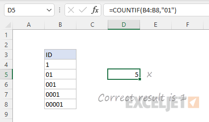
Here the COUNTIF function is set up to count values in B4:B8 that are equal to "01". We expect a result of 1, but COUNTIF returns 5.
=COUNTIF(B4:B8,"01") // returns 5
Somewhere in the calculation process, the leading zeros get dropped and all cells evaluate to 1. This is clearly not the result we want, and shows a limitation of the COUNTIF function. Similarly, if we apply COUNTIF to the worksheet shown above, we get the incorrect result of 4:
=COUNTIF(code,E5) // returns 4
The leading zeros in "009875" are stripped, and 9875 is counted 4 times, when the correct result for "009875"is 2.
Note: COUNTIF is in a group of 8 functions that share some particular quirks and limitations.
SUMPRODUCT solution
A simple solution to this problem is to use the SUMPRODUCT function like this:
=SUMPRODUCT(--(code=E5))
Working from the inside out, we are using the following expression as a logical test:
code=E5
Because code is the named range B5:B16, which contains 12 values, the expression yields 12 TRUE/FALSE results in an array like this:
{FALSE;FALSE;FALSE;TRUE;FALSE;FALSE;FALSE;FALSE;TRUE;FALSE;FALSE;FALSE}
The TRUE values in the array correspond to the cells in B5:B16 that contain "009875". You can see we have TRUE at the fourth cell (B8) and the ninth cell (B13).
Next, we use a double negative (--) to coerce the TRUE/FALSE values to 1s and 0s, which creates the following array:
{0;0;0;1;0;0;0;0;1;0;0;0}
This array is delivered directly to the SUMPRODUCT function, which sums the array and returns a final result:
=SUMPRODUCT({0;0;0;1;0;0;0;0;1;0;0;0}) // returns 2
This is an example of using Boolean algebra in Excel, and you will see many more advanced formulas use this technique. The nice thing about this approach is that it can be easily extended, as explained below.
Sum quantities
As you might have guessed, if you try to use the SUMIF function to sum the quantities associated with code "009875", the same problem will occur. The formula below returns 14, when the correct result is 7:
=SUMIF(code,E5,qty) // returns 14
The cause of the problem is the same: the leading zeros in "009875" get stripped during the SUMIF calculation, which causes "009875" to be grouped together with "9875", and SUMIF sums the quantities associated with both codes.
One of the nicest things about using SUMPRODUCT to perform conditional counts as we did above, is that we can easily extend the logic to perform conditional sums. In this case, all we need to do is multiply the counting logic by the named range qty (C5:C16) like this:
=SUMPRODUCT(--(code=E5)*qty)
This is the formula used in cell G5 of the worksheet. Since we already know that the expression:
--(code=E5)
results in an array of 1s and 0s, we can simplify the formula like this:
=SUMPRODUCT({0;0;0;1;0;0;0;0;1;0;0;0}*qty)
Then, evaluating quantities (qty), we get:
=SUMPRODUCT({0;0;0;1;0;0;0;0;1;0;0;0}*{3;6;4;2;5;6;2;4;5;1;3;3})
After the two arrays are multiplied together we have:
=SUMPRODUCT({0;0;0;2;0;0;0;0;5;0;0;0}) // returns 7
Notice how the zeros in the first array "cancel out" the irrelevant quantities in the second array. In other words, the exact same logic we used to count code "009875" is used to sum quantities associated with code "009875". The final result from SUMPRODUCT is 7.
SUMPRODUCT is a workhorse function that can solve many tricky problems in Excel. See more examples here.
Note: technically the double negative (--) is not needed in the formula to sum quantities above because the math operation of multiplying the two arrays together will automatically coerce the TRUE and FALSE values in the first arrays with 1s and 0s. However, the double negative does no harm and makes the counting and summing formulas easier to compare.