Summary
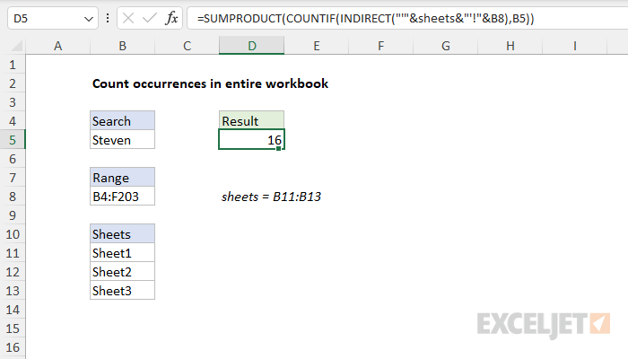
To count total matches across an entire workbook, you can use a formula based on the COUNTIF and SUMPRODUCT functions. In the example shown, the formula in D5 is:
=SUMPRODUCT(COUNTIF(INDIRECT("'"&sheets&"'!"&B8),B5))
where sheets is the named range B11:B13. The result is 16 since there are sixteen occurrences of "Steven" in Sheet1, Sheet2, and Sheet3.
Note: In newer versions of Excel, you can also use the VSTACK function as explained below.
Generic formula
=SUMPRODUCT(COUNTIF(INDIRECT("'"&sheets&"'!"&range),criteria))
Explanation
In this example, the goal is to count the value in cell B5 ("Steven") in the sheets listed in B11:B13. The workbook shown in the example has four worksheets in total. The first sheet is named "Master" and contains the search string, the range, and the sheets to include in the count, as seen in the screenshot above. The next three sheets, "Sheet1", "Sheet2", and "Sheet3" each contain 1000 random first names in the range B4:F203. The table in each sheet looks like this:
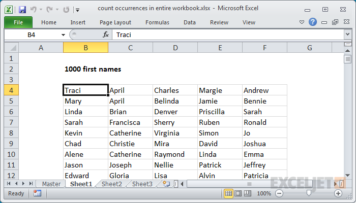
Note that the range (B4:F203) must be adjusted to suit your data.
COUNTIF function
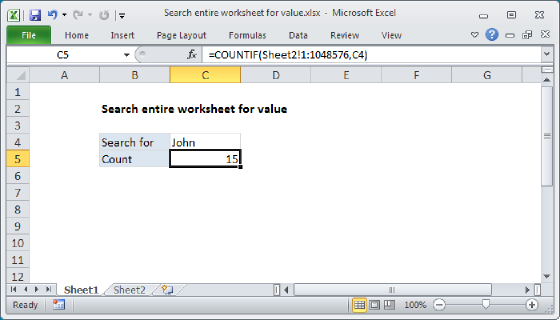
The COUNTIF function returns the count of cells that meet one or more criteria and supports logical operators (>,<,<>,=) and wildcards (*,?) for partial matching. One way to solve this problem is to use the COUNTIF function three times in a formula like this:
=COUNTIF(Sheet1!B4:F203,B5)+COUNTIF(Sheet2!B4:F203,B5)+COUNTIF(Sheet3!B4:F203,B5)
With "Steven" in cell B5, this formula returns 16. This formula works but becomes cumbersome as the number of sheets increases. You might think you could use a 3D reference like this:
=COUNTIF(Sheet1:Sheet3!B4:F203,B5)
However, COUNTIF is in a group of eight functions that have some particular quirks. One of these quirks is that you can't use a 3D reference for the range argument. As a workaround, you can use the INDIRECT function to assemble an array constant, then feed that into COUNTIF. This approach helps streamline the formula as explained below.
COUNTIF with INDIRECT
The INDIRECT function converts a given text string into a proper Excel reference:
=INDIRECT("A1") // returns A1
We can use INDIRECT in this example to create an array constant that contains all three range references as text. In the example shown, the formula in cell D5 is:
=SUMPRODUCT(COUNTIF(INDIRECT("'"&sheets&"'!"&B8),B5))
Working from the inside out, the INDIRECT function is used to assemble a reference to all three ranges like this:
INDIRECT("'"&sheets&"'!"&B8)
Because the named range sheets contains three cells, the code expands like this:
INDIRECT({"'Sheet1'!B4:F203";"'Sheet2'!B4:F203";"'Sheet3'!B4:F203"})
The result in INDIRECT is an array constant that contains three text strings, each representing a range on each of the three sheets. INDIRECT will evaluate the text values and pass the references into COUNTIF as the range argument. For reasons that are somewhat mysterious, COUNTIF will accept the result from INDIRECT without complaint. Because COUNTIF receives more than one range, it will return more than one result in an array like this:
COUNTIF(INDIRECT("'"&sheets&"'!"&B8) // returns {5;6;5}
The code above will return three counts in an array to the SUMPRODUCT function:
=SUMPRODUCT({5;6;5})
With just one array to process, SUMPRODUCT sums the items in the array and returns 16 as a final result. Note that INDIRECT is a volatile function and can impact workbook performance.
VSTACK function
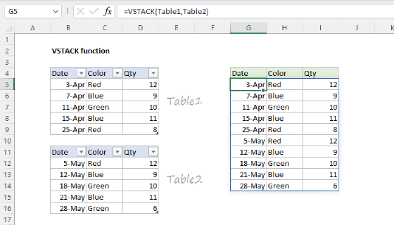
In the current version of Excel, you can use the VSTACK function with a 3D reference to achieve the same result with a more elegant formula:
=SUMPRODUCT(--(VSTACK(Sheet1:Sheet3!B4:F203)=B5))
The VSTACK function combines the three ranges vertically into a single range and feeds the result into the SUMPRODUCT function. Each cell in the combined range is compared to the value in cell B5 ("Steven") resulting in a large array containing only TRUE and FALSE values. We then use a double negative (--) to convert the TRUE and FALSE values into their numeric equivalents, 1 and 0. The numeric array is returned to SUMPRODUCT, which sums all items in the array and returns 16 as a final result. This is an example of using Boolean logic, a common way to solve more complicated problems in Excel.
Note: In Excel 365 and Excel 2021 you can use the SUM function instead of SUMPRODUCT if you prefer in both formulas above. This article provides more detail.