Summary
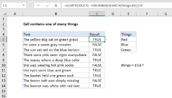
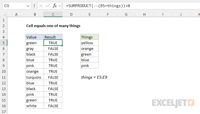
To test if a cell is equal to one of many things, you can use a formula based on the SUMPRODUCT function. In the example shown, the formula in cell C5 is:
=SUMPRODUCT(--(B5=things))>0
where things is the named range E5:E9. The result in cell C5 is TRUE, since "green" is one of the values in E5:E9. As the formula is copied down, it returns a TRUE or FALSE result for each value in column B.
Generic formula
=SUMPRODUCT(--(A1=things))>0
Explanation
In this example, the goal is to return a TRUE or FALSE result for each value in column B, based on whether it appears in the range E5:E9, which has been named "things" for convenience.
Context
Imagine you have a list of values in the range B5:B16 and you want to check each value to see if it appears in another list of values in the range E5:E9, which has been named "things". You might think you can use a formula like this:
=B5=things
However, because we are comparing B5 to the range E5:E9, which contains five values, the formula will return five results. With "green" in cell B5, the result will be an array like this:
{FALSE;FALSE;TRUE;FALSE;FALSE}
And if we copy the formula down, each value in column B will return five results. This idea isn't going to work as-is. You could build a more complicated formula using nested IF statements to check for each value separately, but this is a tricky path that will take much longer and greatly increase the chance of errors. A much simpler, cleaner approach is to use an array formula based on the SUMPRODUCT function.
Solution with SUMPRODUCT
The SUMPRODUCT function multiplies ranges or arrays together and returns the sum of products. This sounds boring, but SUMPRODUCT is a versatile function that can be used to solve many tricky problems in Excel. It works nicely in this case because it can handle arrays natively in any version of Excel.
Note: In Excel 2021 or Excel 365, you can use the SUM function instead of SUMPRODUCT and it will just work fine. However, if the worksheet is opened in an older version of Excel, it will appear as a traditional array formula surrounded by curly braces. If you need backward compatibility, SUMPRODUCT avoids this complication and works the same in all versions.
Back to the problem. As mentioned above, if we compare the value in cell B5 directly with the values in things (E5:E9), we get back an array that contains five TRUE or FALSE values. This seems inconvenient because it isn't obvious how we can resolve this list of five results into a single TRUE or FALSE value. However, we can use SUMPRODUCT to process the array of TRUE/FALSE values and return a single result with a formula like this:
=SUMPRODUCT(--(B5=things))>0
At a high level, this formula counts the TRUE values in the array and then checks if the result is greater than zero. Working from the inside out, the expression B5=things returns five values, as explained above.
=B5=things // returns {FALSE;FALSE;TRUE;FALSE;FALSE}
If we simplify the formula, we now have:
=SUMPRODUCT(--({FALSE;FALSE;TRUE;FALSE;FALSE}))>0
You might wonder what the double negative (--) is doing here. SUMPRODUCT is designed to process numeric values, and it will simply ignore TRUE and FALSE values. If we try to use the raw values, SUMPRODUCT will return zero:
=SUMPRODUCT(FALSE;FALSE;TRUE;FALSE;FALSE}) // returns 0
The double negative (--) is a simple trick to force Excel to convert the TRUE and FALSE values to their numeric equivalents, 1 and 0. After this operation is evaluated, we can simplify the formula to this:
=SUMPRODUCT({0;0;1;0;0})>0
Notice that each FALSE value in the array is now zero, and the lone TRUE in the array is now 1. Now you can see where we are headed. Since the array contains only numbers, SUMPRODUCT will return a sum. If we get any non-zero result, we have a match, so we use >0 to force a final result of either TRUE or FALSE:
=SUMPRODUCT({0;0;1;0;0})>0
=1>0
=TRUE
With a hard-coded list
There's no requirement to use a range for your list of things to check for. If you're only looking for a small number of things, you can use a list in array format, which is called an array constant. For example, if you're just looking for the colors red, blue, and green, you can use {"red","blue","green"} like this:
=SUMPRODUCT(--(B5={"red","blue","green"}))>0
Using a range is a more flexible approach since the values appear on the worksheet and can be changed at any time.
Dealing with extra spaces
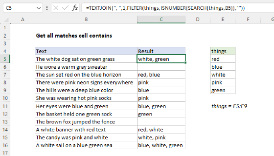
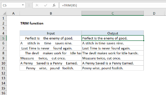
If the cells you are testing contain any extra space, they won't match properly. To strip all extra space, you can modify the formula to use the TRIM function like so:
=SUMPRODUCT(--(TRIM(A1)=things))>0
TRIM will strip leading or trailing space characters from the value before it is compared to the list of things.