Summary
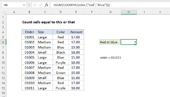
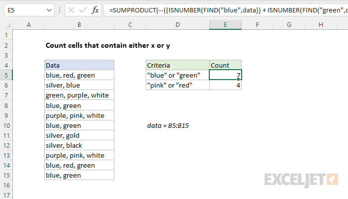
To count cells that contain either x or y, you can use a formula based on the SUMPRODUCT function. In the example shown, the formula in cell E5 is:
=SUMPRODUCT(--((ISNUMBER(FIND("blue",data)) + ISNUMBER(FIND("green",data)))>0))
where data is the named range B5:B15. The result is 7, because there are seven cells in the range B5:B15 that contain "blue" or "green". This formula is case-sensitive because the FIND function is case-sensitive.
Note: It is also possible to use a simpler formula based on a helper column, as explained below.
Generic formula
=SUMPRODUCT(--((ISNUMBER(FIND("abc",range))+ISNUMBER(FIND("def",range)))>0))
Explanation
In this example, the goal is to count cells in the range B5:B15 that contain either "x" or "y", where x and y are both text strings. When you count cells with "OR logic", you need to be careful not to double count. For example, if you are counting cells that contain "blue" or "green", you can't just add together two COUNTIF functions, because you may double count cells that contain both "blue" and "green". The article below explains two options, a single formula based on the SUMPRODUCT function, and a second option based on the COUNTIF function and a helper column. For convenience, the range B5:B15 is named data.
Note: The main formula described on this page is case-sensitive because the FIND function is case-sensitive. If you want a formula that is not case-sensitive, you can substitute the SEARCH function for the FIND function.
SUMPRODUCT formula
One way to solve this problem is to use the SUMPRODUCT function with ISNUMBER + FIND. The formula in E5 is:
=SUMPRODUCT(--((ISNUMBER(FIND("blue",data))+ISNUMBER(FIND("green",data)))>0))
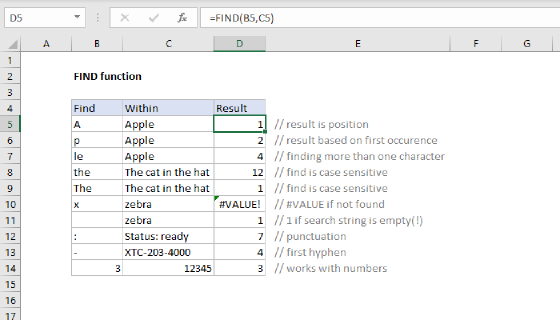
This formula is based on a formula explained here that finds text in a cell. The main work is done with the FIND function and the ISNUMBER function, like this:
ISNUMBER(FIND("red","A red hat") // returns TRUE
FIND returns the number 4 since "red" starts at character 4, and ISNUMBER returns TRUE because 4 is a number. If the text is not found, FIND returns a #VALUE! error and ISNUMBER returns FALSE:
ISNUMBER(FIND("blue","A red hat") // returns FALSE
When given a range of cells, this snippet will return an array of TRUE/FALSE values, one value for each cell in the range. Going back to the formula in the example, and working from the inside out, we look for "blue" like this:
ISNUMBER(FIND("blue",data)
Since the named range data (B5:B15) contains 11 values, we get back an array with 11 TRUE/FALSE values like this:
{TRUE;TRUE;FALSE;TRUE;FALSE;TRUE;FALSE;FALSE;FALSE;TRUE;TRUE}
Each TRUE corresponds to a cell in data that contains "blue". We look for "green" in the same way:
ISNUMBER(FIND("green",data)
And this snippet also returns an array with 11 results:
{TRUE;FALSE;TRUE;TRUE;FALSE;TRUE;FALSE;FALSE;FALSE;TRUE;TRUE}
Next, we add these arrays together with the addition operator (+). The math operation changes the TRUE and FALSE values to 1s and 0s, and the result is a single array:
{2;1;1;2;0;2;0;0;0;2;2}
In this array, a 1 indicates a cell that contains either "blue" or "green" and a 2 indicates a cell that contains both "blue" and "green". Next, we need to add these numbers up, but we don't want to double count. To make sure that any value greater than zero is just counted once, we first force all values to TRUE or FALSE with ">0":
{2;1;1;2;0;2;0;0;0;2;2})>0
This again creates an array of TRUE and FALSE values:
{TRUE;TRUE;TRUE;TRUE;FALSE;TRUE;FALSE;FALSE;FALSE;TRUE;TRUE}
Because we want numbers, we use a double-negative (--) to change the TRUE and FALSE values to 1s and 0s to yield an array like this:
{1;1;1;1;0;1;0;0;0;1;1}
In this array, a 1 indicates a cell in data that contains "blue" or "green" and a 0 indicates a cell that does not contain "blue" or "green". To summarize the operations above:
=SUMPRODUCT(--(({2;1;1;2;0;2;0;0;0;2;2})>0))
=SUMPRODUCT({1;1;1;1;0;1;0;0;0;1;1})
Finally, SUMPRODUCT returns the sum of all values in the array, 7, as a final result.
Note: this formula is an example of using Boolean algebra to apply "OR logic" in a formula.
Helper column solution
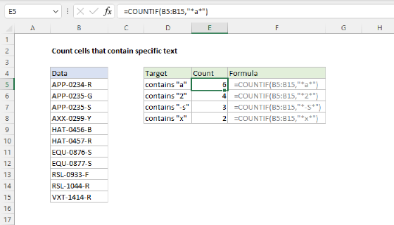
Another way to solve this problem is with a helper column. This breaks up a more complex problem into parts. To check each cell in B5:B15 for "blue" or "green", we can use the COUNTIF function with an array constant like this:
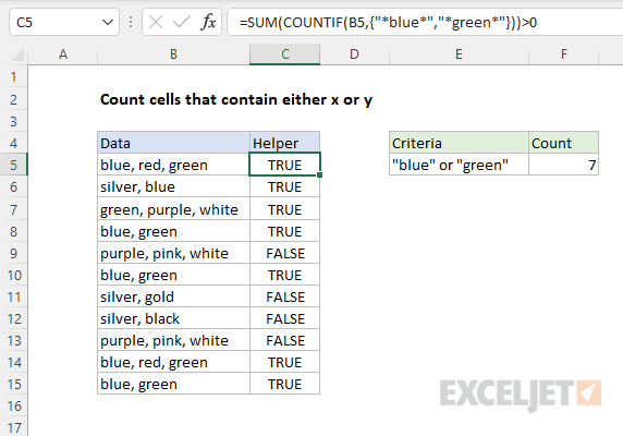
=SUM(COUNTIF(B5,{"*blue*","*green*"}))>0
Because we give COUNTIF an array that contains two items for criteria, it returns an array that contains two counts: one for "blue" and one for "green". The asterisk (*) is a wildcard we can use for a contains search. To prevent double counting, we add the counts up with the SUM function and then force the result to TRUE/FALSE with ">0". As the formula is copied down, we get a TRUE or FALSE value in column C for each value in column B.
This is how the helper column looks on the worksheet:
To sum up all TRUE in C5:C15, we can use the SUMPRODUCT function. The formula in F5 is:
=SUMPRODUCT(--C5:C15)
The double negative (--) coerces the TRUE and FALSE values to 1s and 0s:
=SUMPRODUCT({1;1;1;1;0;1;0;0;0;1;1}) // returns 7
and SUMPRODUCT returns 7 as a final result.