Summary
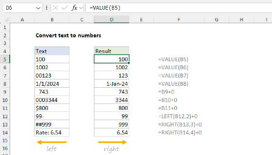
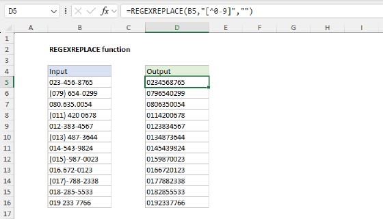
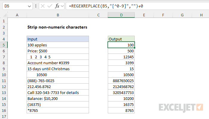
To remove all non-numeric characters from a text string, you can use a formula based on the REGEXREPLACE function. In the example shown, the formula in D5 is:
=REGEXREPLACE(B5,"[^0-9]","")+0
As the formula is copied down, REGEXREPLACE removes all characters except the digits between 0-9 from the text strings in column B, when we add zero (+0) to make Excel convert the result to a numeric value.
Note: REGEXREPLACE is available in Excel 365. For older versions of Excel, see below.
Generic formula
=REGEXREPLACE(A1,"[^0-9]","")+0
Explanation
In this example, the goal is to strip (i.e., remove) non-numeric characters from a text string with a formula. Until 2024, this was a tricky problem in Excel, partly because Excel did not support regex (Regular Expressions), and partly because there wasn't a good way to convert a text string into an array of characters where they could be easily processed with other functions. However, with the introduction of Regular Expressions in Excel in late 2024, the problem became much simpler. In the article below, we look first at the REGEXEXTRACT function, then we explore more complex ways of accomplishing the same thing in older versions of Excel.
Note: Adding zero (+0) is a trick to convert text into numbers. Read more here.
Table of contents
Excel 365
In Excel 365, we now have formula support for Regular Expressions in the form of three new functions: REGEXTEST, REGEXEXTRACT, and REGEXREPLACE. This drastically simplifies the problem because we can easily use a regex pattern like [^0-9] to target non-numeric characters. One way to do this is to use the REGEXREPLACE function to match non-numeric characters and replace them with an empty string (""). This is the approach used in the worksheet shown, where the formula in D5 looks like this:
=REGEXREPLACE(B5,"[^0-9]","")+0
The REGEXREPLACE function replaces text matching a specific regex pattern in a given text string. In this problem, we configure REGEXREPLACE as follows:
- text - the text to process (B5)
- pattern - the pattern to use when matching text ([^0-9])
- replacement - the text to use for replacing matches
The power of this formula comes from the pattern [^0-9], which can be roughly translated to "match anything that is NOT a digit from 0 to 9." The meaning breaks down like this:
- The square brackets [ ] create what's called a "character class" - a group of characters to match
- The caret ^ at the beginning inside the brackets means "NOT" - it negates everything that follows
- 0-9 represents all digits from 0 to 9
- So together, [^0-9] tells the regular expression engine: "Find any character that is not a digit."
When we use [^0-9] with the replacement text ", we are saying: "Find any character that's not a number and replace it with nothing," - which leaves only the numbers behind. It's a bit like a sieve that only lets numbers pass through while filtering out everything else.
The last step in the formula is to change the text result from REGEXREPLACE, which always returns a text string, into a proper number. In this instance, we do this by adding zero. This is a short way of forcing Excel to try and evaluate the text as a number without changing the number. The VALUE function is another way to do the same thing.
Preserving the decimal point
If you have numbers with decimal places, you can adjust the formula as follows to also keep the period (.) character:
=REGEXREPLACE(B5,"[^0-9.]","")+0
The only change is adding the period (.) to the pattern [^0-9.] inside the square brackets.
Older versions of Excel
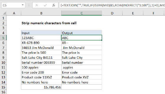
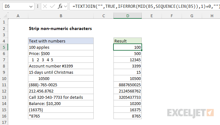
In older versions of Excel, this is a harder problem to solve. The solutions described below involve converting the text string to an array of characters and then removing non-numeric characters before joining things together again with TEXTJOIN. The screen below shows one approach:
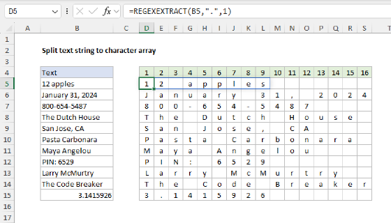
Creating an array of characters
Working from the inside out, the first step in this problem is to create an array of characters from the text string in column B. This is done with the snippet of code below:
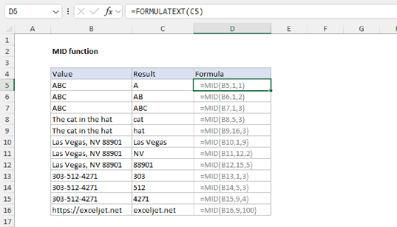
MID(B5,SEQUENCE(LEN(B5)),1)
First, the LEN function runs and returns a count of 10, since there are 10 characters in the text string "100 apples". This result is returned to the SEQUENCE function as the rows argument:
MID(B5,SEQUENCE(10),1)
Next, SEQUENCE generates a numeric array of the numbers 1-10, which is returned to the MID function as the start_num argument:
MID(B5,{1;2;3;4;5;6;7;8;9;10},1)
This is the current solution for creating an array of characters in an Excel formula. In this configuration, the MID function extracts the text in B5, one character at a time, and returns an array that looks like this:
{"1";"0";"0";" ";"a";"p";"p";"l";"e";"s"}
We now have an array that contains all characters in cell B5. The next step is to figure out which characters are numbers.
Testing for numeric values
Since we have an array of characters ready to go, you might think we can just pass them into the ISNUMBER function like this:
=ISNUMBER(array)
The problem, though, is that the numbers in the array (if any) are actually represented as text values like "1", "0", etc. If we try to use ISNUMBER like this, it will return FALSE for every character! One solution is to use a small hack to "force" Excel to convert numbers by adding zero. A math operation like this Excel to try to convert the character to a number. Adding zero to a non-numeric character like "a", will result in a #VALUE! error. However, adding zero to "1" will convert "1" to the number 1:
="a"+0 // returns #VALUE!
="1"+0 // returns 1
This is the trick used in the formula, where we add zero to the array of characters returned by the MID function:
{"1";"0";"0";" ";"a";"p";"p";"l";"e";"s"}+0
Because the array contains 10 characters, we get back an array of 10 results like this:
{1;0;0;#VALUE!;#VALUE!;#VALUE!;#VALUE!;#VALUE!;#VALUE!;#VALUE!}
Notice that only the first 3 characters have survived this operation (since they are numbers), and the remaining characters are now #VALUE! errors. This is the final piece we need to remove the non-numeric characters.
Removing non-numeric characters
The way we remove non-numeric characters in this formula is also tricky - we use the IFERROR function like this:
IFERROR(MID(B5,SEQUENCE(LEN(B5)),1)+0,"")
By wrapping a formula in IFERROR, we force another result when the formula returns an error. When the formula does not return an error, the result passes through IFERROR unchanged. The snippet uses this behavior to convert errors to an empty string (""). After the IFERROR function processes the array returned by MID, it returns an array like this:
{1;0;0;"";"";"";"";"";"";""}
Notice the #VALUE! errors are now gone, replaced by empty strings. At this point, the remaining task is to assemble the remaining numbers into a final numeric value.
Creating the final numeric value
The last step in this problem is to join the surviving numeric values into a single number. The tool we use to perform this step is the TEXTJOIN function, which is designed to concatenate values in a range or array. In this formula, the result from IFERROR is returned to TEXTJOIN as the text1 argument like this:
=TEXTJOIN("",TRUE,{1;0;0;"";"";"";"";"";"";""})
Notice that we provide delimiter as an empty string ("") because we don't want any extra characters in the final result and we supply TRUE for ignore_empty because we don't want to include the empty strings in the final result. In this configuration, TEXTJOIN returns the three numbers in a text string like this:
="100"
So close! But notice we again have a text value because TEXTJOIN performs concatenation, which always results in a text string. The final step is to again add zero to force Excel to convert the text to a number:
="100"+0 // returns 100
Note: if you prefer, you can use the VALUE function instead of adding a zero to convert numbers as text values into numeric values. Adding zero is just a shortcut.
A better formula?
After I finished documenting the formula above, upgrading it to use the SEQUENCE function, I realized that a better approach is probably to use the FILTER function with the LET function like this:
=LET(
chars,MID(B5,SEQUENCE(LEN(B5)),1),
TEXTJOIN("",1,FILTER(chars,ISNUMBER(chars+0)))+0
)
FILTER is a more natural solution because it is designed to filter out unwanted values. The catch though is that we need to use the character array created by MID + SEQUENCE more than once, which means we should introduce the LET function for efficiency. In the formula above, we store the result from MID in a variable named "chars", then we use that variable twice inside FILTER like this:
=FILTER(chars,ISNUMBER(chars+0))
Inside the include argument of FILTER we add zero to the array to force Excel to try to convert the characters to numbers. As explained above, chars + 0 will return an array like this:
{1;0;0;#VALUE!;#VALUE!;#VALUE!;#VALUE!;#VALUE!;#VALUE!;#VALUE!}
Then, the ISNUMBER function will return an array like this:
{TRUE;TRUE;TRUE;FALSE;FALSE;FALSE;FALSE;FALSE;FALSE;FALSE}
The final result from FILTER is an array that contains just the three numbers:
{"1";"0";"0"}
We then join the numbers with TEXTJOIN and (again) force a numeric result by adding zero:
=TEXTJOIN("",1,{"1";"0";"0"})+0
="100"+0
=100
The final result is 100, the same as before. This formula is slightly more verbose than the original, but it is easier to adapt to filter characters in different ways. For example, if you want to preserve decimal points or periods (.), you could adjust the formula like this:
=LET(
chars,MID(D37,SEQUENCE(LEN(D37)),1),
TEXTJOIN("",1,FILTER(chars,ISNUMBER(chars+0)+(chars=".")))+0
)
The original formula is shorter but more cryptic and works best for the intended task only.
Excel 2019
If you happen to be using Excel 2019, which provides the TEXTJOIN function but not the SEQUENCE function, you can use an alternative formula like this:
=TEXTJOIN("",TRUE,IFERROR(MID(B5,ROW(INDIRECT("1:"&LEN(B5))),1)+0,""))
Note: In Excel 2019 this is an array formula and must be entered with control + shift + enter.
The ROW + INDIRECT construction is another way in older versions of Excel to create a numeric array with a variable length:
=ROW(INDIRECT("1:"&LEN(B5))
=ROW(INDIRECT("1:"&10))
=ROW(INDIRECT("1:10"))
={1;2;3;4;5;6;7;8;9;10}
The resulting array is the same as that returned by the SEQUENCE function above. Note that INDIRECT is a volatile function that can cause performance problems so this approach should be avoided in later versions of Excel.
Strip numeric characters
To remove numeric characters from a text string use the formulas explained here.