Summary
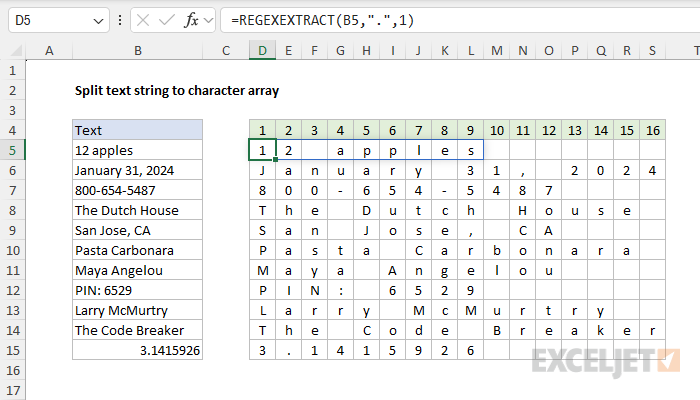
To convert a text string into an array of characters, you can use a simple formula based on the REGEXEXTRACT function. In the example shown, the formula in cell D5 is:
=REGEXEXTRACT(B5,".",1)
The result is a horizontal array containing the 9 characters in "12 apples" that spills into the range D5:L5. As the formula is copied down, each text string in column B is converted to an array of characters.
REGEXEXTRACT is a new function in Excel 365. The article below describes some alternatives that will work in older versions of Excel.
Generic formula
=REGEXEXTRACT(text,".",1)
Explanation
In this example, the goal is to use a formula to split a text string into an array of characters. For example, if the text string is "Apple", the resulting array should be {"A","p","p","l","e"}. For a long time, this was quite a difficult problem that required a complicated array formula approach. When the SEQUENCE function was introduced, the problem became simpler since SEQUENCE could generate numbers that could be used with the MID function to extract characters one by one. The big breakthrough, however, came when the REGEXEXTRACT function was introduced. For the first time in Excel, you can convert a text string to an array of characters with a single function call. The article below explains several options for solving this problem, including options that will work in older versions of Excel.
Why create an array of characters?
Why would you want to convert a text string to an array? Basically, an array is a convenient container that you can feed into many other functions. Remember that arrays in Excel correspond directly to ranges, and there are many Excel functions designed to work with arrays and ranges. Once you have content in an array, you apply functions to sort, filter, count, analyze, extract unique values, etc. For example, you could use the FILTER function to preserve or remove specific characters and then use the TEXTJOIN function to recombine the remaining characters into a text string. Here are some scenarios where splitting a text string into an array of characters can be useful:
- To remove specific characters in a text string with the FILTER function.
- To sort characters in a text string with the SORT function.
- To count unique characters in a text string with the UNIQUE function.
- To process characters with the CODE or UNICODE function.
Why not TEXTSPLIT?
The newer TEXTSPLIT function is designed to split text strings into arrays using a custom delimiter. TEXTSPLIT works great for splitting text into words or splitting comma-separated text. However, there is currently no way to split text into characters with TEXTSPLIT because there is no "delimiter" between characters. You might think you can do something clever like this:
=TEXTSPLIT(A1,"")
But that won't work. TEXTSPLIT will return a #VALUE! error.
Option #1 - REGEXEXTRACT
In 2024, Excel introduced the REGEXEXTRACT function and this provides the simplest and cleanest way to convert a text string to an array of characters. This is the method used in the workbook shown above, where the formula in D5 looks like this:
=REGEXEXTRACT(B5,".",1)
The configuration for REGEXEXTRACT is simple:
- text - provided as B5
- pattern - provided as "." (in regex, this means "any single character")
- return_mode - provided as 1 (all matches)
In cell D5, the REGEXEXTRACT function returns an array of 9 characters like this:
{"1","2"," ","a","p","p","l","e","s"}
As the formula is copied down, it returns a character array for each of the text strings seen in column B. As you can see, this is a simple and elegant solution. I recommend this approach if you have access to REGEXEXTRACT.
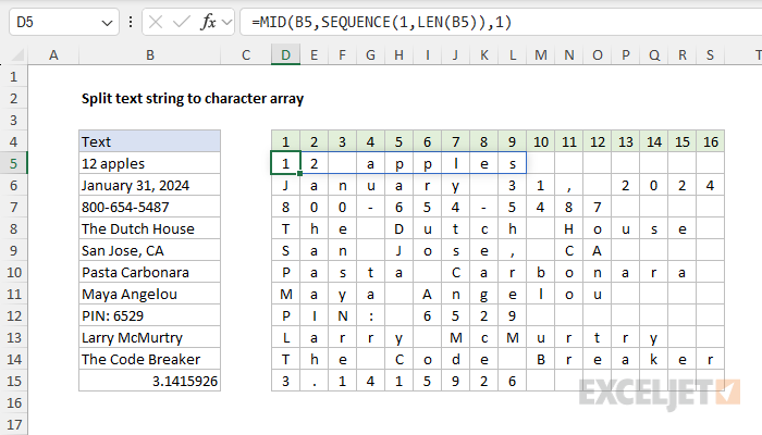
Option #2 - MID and SEQUENCE
Before the REGEXEXTRACT function became available in Excel, the best way to solve this problem was to use a formula based on the MID, SEQUENCE, and LEN functions. You can see this approach below, where the formula in D5 is:
=MID(B5,SEQUENCE(1,LEN(B5)),1)
Essentially, this is a workaround formula. To understand this formula, we need to consider how the MID function is designed to work. Typically, the MID function is used to extract one or more characters from a text string with a syntax like this:
=MID(text,start_num,num_chars)
For example, you can use MID like this:
=MID("12 apples",1,1) // returns "1"
=MID("12 apples",1,2) // returns "12"
=MID("12 apples",3,6) // returns "apple"
Depending on the value given for start_num and num_chars, we get a different part of the string. However, in this case, we don't want to return parts of the text string; we want to return all the characters in the text string together in an array. The trick is to ask the MID function for more than one start_num simultaneously. For example, to return the three letters in "red" in an array, we can use the array constant {1,2,3} like this:
=MID("red",{1,2,3},1) // returns {"r","e","d"}
Because we are asking MID for 1 character starting at three positions {1,2,3}, we get back all three letters in "red" in a single array. This approach works, but we need a way to generate the numeric sequence dynamically. Enter the SEQUENCE function, which is perfectly suited for this task. Turning back to the example above, we have this formula in cell D5:
=MID(B5,SEQUENCE(1,LEN(B5)),1)
Working from the& inside out, the LEN function is used to calculate the number of characters in cell B5, which is 9. Dropping that value into the formula, we have:
=MID(B5,SEQUENCE(1,9),1)
With 1 for the rows argument and 9 for columns, SEQUENCE returns a numeric array beginning with 1 and ending with 9. This array is delivered to the MID function as the start_num, with num_chars set to 1:
=MID(B5,{1,2,3,4,5,6,7,8,9},1)
In other words, we are asking MID for 1 character starting at nine different positions, one for each character in the source text. With this configuration, MID dutifully extracts all 9 characters in delivers the result in an array like this:
{"1","2"," ","a","p","p","l","e","s"}
When this array lands in cell D5, it spills into the range D5:L5. Notice the final array is comma-separated, which corresponds to a horizontal array or range in Excel. The reason we get a horizontal array in columns instead of a vertical array in rows is that we configured SEQUENCE to ask for columns instead of rows.
This formula is more transparent than the REGEXEXTRACT option. It is possible to understand what the formula is doing step-by-step. However, it is also significantly more complex.
Legacy Excel
In Legacy Excel, it is more challenging to split a text string into an array of characters. There are two basic approaches. The first and easiest is to use carefully constructed mixed references in a worksheet that has the numbers you need already available. The second approach is to use a more complex array formula.
Option #1 - MID + Mixed references
If the goal is to extract characters into separate cells, you can use a simple formula that relies on mixed references. The trick is to set up a worksheet that contains a sequence of numbers that can be used to extract characters one by one with the MID function. You can see this approach below, where the formula in D5 looks like this:
=MID($B5,D$4,1)
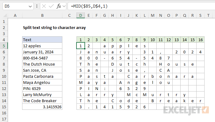
This works because we can use the numbers in the range D4:P4 directly as start_num inside the MID function. Notice that $B5 and D$4 are both mixed references so that the formula can be copied throughout the range. Compared to the dynamic array solution above, one big difference in this approach is that results will not automatically spill onto the worksheet into a spill range. Instead, the formulas must be manually copied into a range of cells big enough to hold all characters.
Option #2 - Array formula with INDIRECT + ROW
There is a way to generate an array of characters from a text string in older versions of Excel, but it requires a more complicated array formula. The core of this solution is to use the ROW and INDIRECT functions in place of SEQUENCE like this:
=MID(B5,ROW(INDIRECT("1:"&LEN(B5))),1)
You will find code like this in many older array formulas that predate dynamic arrays in Excel. The INDIRECT function is a way of changing cell references as text into actual cell references. In the formula above, INDIRECT converts the text "1:9" into an actual reference, and ROW returns an array of row numbers. The code evaluates like this:
=MID(B5,ROW(INDIRECT("1:"&LEN(B5))),1)
=MID(B5,ROW(INDIRECT("1:"&9)),1)
=MID(B5,ROW(INDIRECT("1:9")),1)
=MID(B5,{1;2;3;4;5;6;7;8;9},1)
={"1";"2";" ";"a";"p";"p";"l";"e";"s"}
One problem with the formula above is that the array is vertical because we are using the ROW function. To get a horizontal array, the last step is to wrap the formula in the TRANSPOSE function like this:
=TRANSPOSE(MID(B5,ROW(INDIRECT("1:"&LEN(B5))),1))
The final result is a horizontal array, as you can see in the worksheet below:
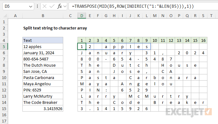
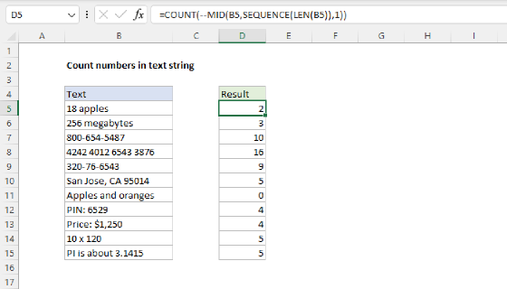
Unfortunately, this array formula won't spill in older versions of Excel, and it requires special handling. To make it work, you must first select the correct number of cells (D5:L5 in row 5), then enter the formula as a multi-cell array formula. This makes the formula unworkable if you need automation. However, this approach still has value in older versions of Excel in formulas that don't need to spill multiple values. For an example, see Count numbers in a text string.