Summary
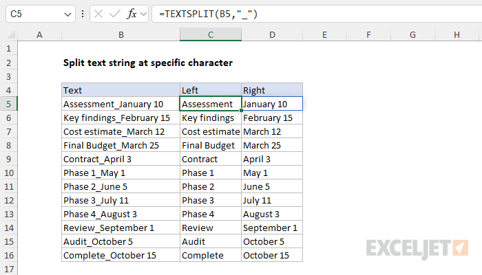
To split a text string at a specific character with a formula, you can use the TEXTSPLIT function. In the example shown, the formula in C5 is:
=TEXTSPLIT(B5,"_")
As the formula is copied down, it returns the results seen in columns C and D.
Note: If you are using an older version of Excel that does not offer the TEXTSPLIT function, you can use a formula based on the LEFT, RIGHT, LEN, and FIND functions as explained below.
Generic formula
=TEXTSPLIT(A1,"_")
Explanation
In this example, the goal is to split a text string at the underscore("_") character with a formula. Notice the location of the underscore is different in each row. This means the formula needs to locate the position of the underscore character first before any text is extracted. There are two basic approaches to solving this problem. If you are using Excel 365, the best approach is to use the TEXTBEFORE and TEXTAFTER functions. If you are using an older version of Excel without these functions, you can use a more complicated formula that combines the LEFT, RIGHT, LEN, and FIND functions. Both approaches are explained below.
Note: in the worksheet shown, we split text at the underscore character ("_"), but the solutions below can be adapted to split text at any character.
How to split text in Excel 365
The current version of Excel 365 contains three new functions that make this problem quite simple:
- TEXTSPLIT function - split text at all given delimiters
- TEXTBEFORE function - get the text before a specific delimiter
- TEXTAFTER function - get the text after a specific delimiter
Each option is described below. Choose the best option based on your specific needs.
TEXTSPLIT function
The TEXTSPLIT function splits text at a given delimiter and returns the split text in an array that spills onto the worksheet into multiple cells. In the worksheet shown, the formula used to split text in cell C5 is:
=TEXTSPLIT(B5,"_")
The text comes from cell B5 and the delimiter is provided as the underscore character wrapped in double quotes ("_"). The result is an array with two values like this:
{"Assessment","January 10"}
This array lands in cell C5 and spills into the range C5:D5. The result is "Assessment in cell C5 and "January 10" in cell D5. As the formula is copied down it performs the same operation on all values in column B.
Video demo: Excel TEXTSPLIT function
With TEXTBEFORE and TEXTAFTER
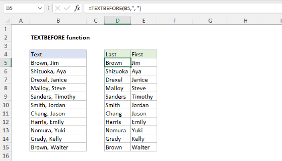
Another way to solve this problem is to use the TEXTBEFORE and TEXTAFTER functions separately. You can extract text on the left side of the underscore with the TEXTBEFORE function in cell C5 like this:
=TEXTBEFORE(B5,"_") // left side
As the formula is copied down, it returns the text before the underscore for each text string in B5:B16.
Video demo: Excel TEXTBEFORE function
To extract text on the right side of the underscore, use the TEXTAFTER function in cell D5 like this:
=TEXTAFTER(B5,"_") // right side
As the formula is copied down, it returns the text after the underscore for each text string in B5:B16.
Video demo: Excel TEXTAFTER function
How to split text in an older version of Excel
Older versions of Excel do not offer the TEXTSPLIT, TEXTBEFORE, or TEXTAFTER functions. However, you can still split text at a specific character with a more complex formula that combines the LEFT, RIGHT, LEN, and FIND functions.
Left side
To extract the text on the left side of the underscore, you can use a formula like this in cell C5:
LEFT(B5,FIND("_",B5)-1) // left
Working from the inside out, this formula uses the FIND function to locate the underscore character ("_") in the text, then subtracts 1 to move back one character:
FIND("_",B5)-1 // returns 10
FIND returns 11, so the result after subtracting 1 is 10. This result is fed into the LEFT function as the num_chars argument, the number of characters to extract from B5, starting from the first character on the left:
=LEFT(B5,10) // returns "Assessment"
The LEFT function returns the string "Assessment" as the final result. As this formula is copied down, it will return the same results seen in column C above.
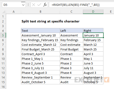
Right side
To extract text on the right side of the underscore, you can use a formula like this in cell D5:
RIGHT(B5,LEN(B5)-FIND("_",B5)) // right
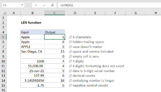
As above, this formula also uses the FIND function to locate the underscore ("_") at position 11. However, in this case, we want to extract text from the right side of the string, so we need to calculate the number of characters to extract from the right. This is done by subtracting the result from FIND (11) from the total length of the text in B5 (21), which is calculated with the LEN function:
=LEN(B5)-FIND("_",B5)
=21-11
=10
The result is 10, which is returned to the RIGHT function as num_chars, the number of characters to extract from the right:
=RIGHT(B5,10) // returns "January 10"
The final result in D5 is the string "January 10". As this formula is copied down, it will return the same results seen in column D above.